2D Distance fields and Voronoi maps
Introduction
Let us consider the following distance field problem: given a domain $\mathcal{D}$ in 2D (subset of $\mathbb{Z}^2$) and a set of sites $\mathcal{S}$ (also in $\mathcal{D}$), we would like to compute, for each point in $\mathcal{D}$, its closest point in $\mathcal{S}$ for the Euclidean metric. Such map defines the distance transformation (or distance map, or distance field) of $\mathcal{S}$.
![]()
This distance information has many applications in a huge number of applications, e.g. for shape analysis, shape matching, rendering, medial axis extraction, implicit function based CSG, modeling for fabrication, numerical algorithms for PDE solving… just to name few of them.
![]()
In this document, the objective is to focus on the algorithmic aspects of the distance transform computations, describing a fast, generic and parallel algorithm. First, let’s observe that computing the distance transform and the Voronoi diagram $\mathcal{V}$ of $\mathcal{S}$ restricted to $\mathcal{D}$ are similar problems: from the Voronoi map ($\mathcal{V}\cap\mathcal{D}$), the distance transform is obtained by computing the distance of each point to the site of the cell it belongs to.

Before diving into the algorithmic details, a first naive algorithm can be sketched as follows:
for each point p  in D
 mindist = infinity
 for each point q in S
   mindist = min( mindist, ||p - q||_2 )
with a very expensive computational cost in $O(|\mathcal{S}|\cdot|\mathcal{D}|)$. One can use a generic Voronoi diagram algorithm and then locate each grid point in $\mathcal{D}$ in $\mathcal{V}$. This would lead to a $O( |\mathcal{S}|\log{|\mathcal{S}|} + |\mathcal{D}|\log{|\mathcal{S}|})$ algorithm. We describe below an optimal and exact $\Theta(|\mathcal{D}|)$ algorithm which corresponds to an ad-hoc separable construction of the Voronoi map.
Related works
Before describing the details, we review the huge literature on the subject. To design efficient algorithms, some authors have considered the exact solution with approximation of the Euclidean metric (e.g. using Chamfer masks, or other path based-metrics), or approximated solutions using the Euclidean metric (e.g. vector propagation, or the GPU-friendly Jump Flooding Algorithm). One of the first exact distance transform algorithms have been proposed by [Breu et al 1995], [Saito and Toriwaki 1996] and [Hirata 1996]). The linear in time algorithm described below follows [Maurer et al 2003]. In the literature, many derivatives or variants of this idea exist.
Fast Separable Algorithm
Warm-up
The first key feature of the approach relies on the separability property of the distance transform computation. This is due to a monotinicity propoerty of the Euclidean distance function. A way to illustrate this is to consider the following distance problem for $p(i,j)\in\mathcal{D}$: $$dt(p) = argmin_{q\in\mathcal{S}} ( ||p-q||2 ) =argmin{(u,v)\in\mathcal{S}} ( (i - u)^2 + (j-v)^2),$$ which can be rewritten as a first series of independent 1D minimizations along the first dimension of the domain: $$dt_X(i,j) = \min_{(u,j)\in\mathcal{S}} ( (i-u)^2)$$ followed by another series of 1D minimizations along the second dimension to get the final result: $$dt(i,j) = \min_{(i,v)\in\mathcal{S}} ( dt_X(i,v) + (j-v)^2),$$ and so forth for extra dimensions for higher dimensional problems. See below for a discussion on the class of metrics for which such property holds.
As Voronoi map and Euclidean distance transform are closely related, similar separable approach will be used for the Voronoi map extraction problem, solving each 1D subproblem in $\Theta(n)$ for $\mathcal{D}=[0,n)\times[0,n)$.
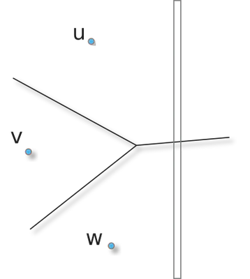
The first step
Let us consider this small example (sites $\mathcal{S}$ are in blue):

For each row, independently, let’s compute the partial 1D Voronoi map (one color per Voronoi cell):

This can be done by a simple $O(n)$ propagation: a first scan from left to right to discover the sites in the row and a rewritting step to label each pixel (boundary of Voronoi cell being the mid-point between each two consecutive sites).
On an $[0,n)\times[0,n)$ domain, this first step can be done in $\Theta(n^2)$.
The second step
To illustrate the second step (along each column independently), let us consider the following example:
| input | result after the first step |
|---|---|
 |
 |
Let us consider a column. From the first step, we have, at each point,
| the closest site in each row:

To obtain the resulting Voronoi map on that column, we need to filter
out sites whose Voronoi cell does not intersect the vertical slab. To
perform that efficiently, we can rely on an hiddenBy(u,v,w, slab)
predicate which returns true if the Voronoi cell of v does not intersect
the slab (vertical column here), given the sites u and w
($u_y>v_y>w_y$). For the Euclidean metric, this can be decided in $\Theta(1)$.
The algorithm can be sketched as follows: we start with three
sites for which the hiddenBy predicate is false (in a given top-down
or bottom-up order) and stored in a stack. We add sites one by one and
we check the predicate on the top three sites of the stack. If
true, it means that the new site hides previous ones and the
middle site is popped out. The correctedness of the algorithm relies on the monotonicity property
of the Euclidean metric
([Hirata 1996],
[Maurer et al 2003]): For $u,v,w\in S$ with $u_y>v_y>w_y$, if the hiddenBy predicate is true, then $v$ can be safely removed from the Voronoi map subproblem on the slab. As each site in inserted only once,
popped at most once, and since the hiddenBy is in $\Theta(1)$,
pruning the sites along the column of size $n$ can be done in $\Theta(n)$.

The last step consists in rewriting the column with the proper label using a
simple closest(u,v,p) predicate which returns the closest site (u
or v) to a point p in the slab (also in $\Theta(n)$ for a given column).
If we apply this process for all columns, we end up with this Voronoi map:

The Code
Overview
The code in dimension 2 is available in the github project: VoronoiMap2D. The code is meant to be easy to read / adapt / reuse in other contexts. We showcase a multithread (using openmp) Voronoi map computation and distance transformation for the $l_2$ metric.
| Input | Output Voronoi map | Output distance transformation |
|---|---|---|
 |
 |
 |
For such metric, the closest and hiddenBy predicates end up to be the following simple c++ lambdas (see the code for the generic Image class and the site coordinates encoding):
 auto closest = [&source](const Index x, const Index y,
                          const Index siteA, const Index siteB)
  {
    auto sAx=source.getX(siteA), sAy=source.getY(siteA);
    auto sBx=source.getX(siteB), sBy=source.getY(siteB);
    return (x-sAx)*(x-sAx) + (y-sAy)*(y-sAy) > (x-sBx)*(x-sBx) + (y-sBy)*(y-sBy);
  };

  auto hiddenBy = [&source](const Index A, const Index B, const Index C,
                            const Index slabX)
  {
    auto sAx=source.getX(A), sAy=source.getY(A);
    auto sBx=source.getX(B), sBy=source.getY(B);
    auto sCx=source.getX(C), sCy=source.getY(C);
    int a,b,c;
    a = sBy - sAy;
    b = sCy - sBy;
    c = a + b;
    int dA=(sAx-slabX)*(sAx-slabX), dB=(sBx-slabX)*(sBx-slabX), dC=(sCx-slabX)*(sCx-slabX);
    return (c * dB -  b*dA - a*dC - a*b*c) > 0 ;
  };
Multithreading
At the first and second steps, in each 1D subproblem, we need to propagate quantities which may be difficult to parallelize. However, as 1D subproblems are independent in each step, it is straightforward to solve each 1D subproblem in parallel and to gather the result before going to the next step.
For example, using four shared memory threads, one can split the problem into four independent processes of two 1D subproblems along the rows, synchronize the threads and then four independent processes again across the columns:

In the code example, a single openmp macro on the outer for loop for each step is used to parallelize the Voronoi map extraction.
Further reading and extensions
Few concluding remarks:
- The algorithm can be trivially extended to higher dimensions. E.g. in 3D, we just have to repeat the
hiddenByfiltering along the third z dimension. Please refer to DGtal for a multithread implementation in arbitrary dimensions. - For the $l_2$ metric,
closestandhiddenBypredicates are in $O(1)$ and for a Voronoi map extraction problem in dimension $d$, i.e. $[0,n)^d$ domain, the overall separable approach is in $O(dn^d)$ (first step + $(d-1)$ second step). - Similar separable approach can be used to compute the Power Diagram of a set of weighted points and the discrete medial axis Ref, also available in DGtal.
- The class of metrics for which the algorithm output exact Voronoi map is quite large. For instance, any (weighted) $l_p$ metric can be considered (for $p\geq1$) or a large class of path based norms (see DGtal doc page and Ref). The only difference is to provide an implementation of the
closestandhiddenBypredicates for the metric (which may not be in $O(1)$, thus impacting the overall computational cost).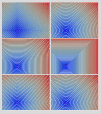
- For example, for $l_p$ metrics with $p\geq 1 \in\mathbb{N}$, the
closestpredicate can be implemented in $O(d\log{p})$ (using exponentiation by squaring). ThehiddenByone can be designed in $O(d\log{n}\log{p})$, leading to an overall cost in $O(d^2n^d\log{p}\log{n})$. - Using a simple update of the code, it can also handle periodic –toroidal– domains.
- The described algorithm can be adapted to compute the Voronoi map with all cocyclic points (exactly $\mathcal{V}\cap\mathbb{Z}^2$) with a small computational overhead (e.g. Ref).
- In both steps, we have to perform some propagation across 1D domains, which could be difficult to efficiently implement them on GPU. Addressing this issue, we can mention the parallel banding approach for the exact distance transformation computation.
- On a more theoretical side, [Ref] describes an $O(\log{n})$ separable algorithm on an EREW computational model (with $O(n^2/\log\log{n})$ processors).