Digital Geometry in Computer Graphics
David Coeurjolly
CNRS,
Université de Lyon

Digital Geometry model and applications
Digital geometry model in one slide
Topology and geometry processing of objects defined on regular lattices
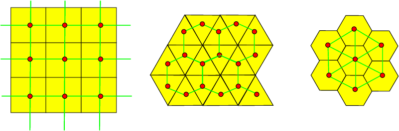
- Digital Objects = subsets of $\mathbb{Z}^d$
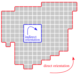
- Digital Topology = adjacency relationship induced by the lattice
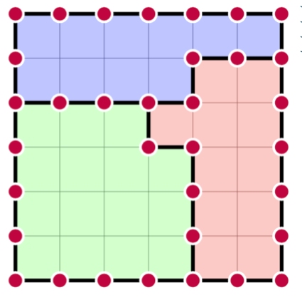
- Digital surfaces = cells of a Cartesian cubical complex
- Geometrical predicates = integer only computations
- Fundamental objects (straight lines, circles...) = constructive approach or as the digitization of Euclidean ones
Motivations
|
|  |
$\Rightarrow$ no interpolation/approximation | 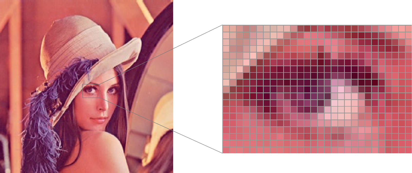 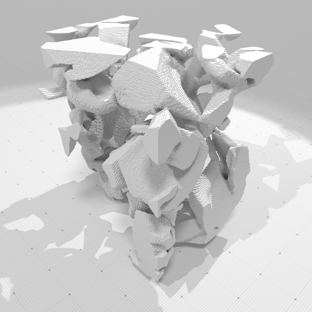 |
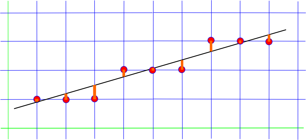
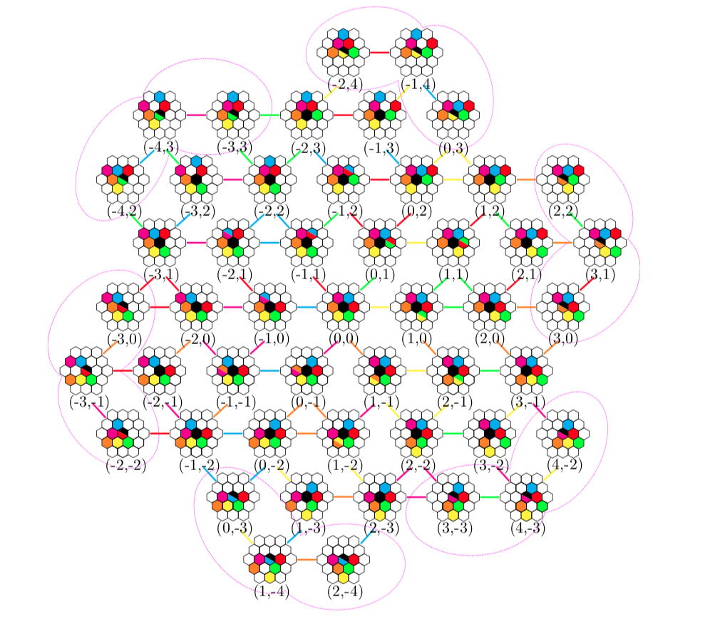
Arithmetic in DG: straight lines
|
$y= \alpha\cdot x$, |
$\alpha$ is rational $\frac{p}{q}$ $\Rightarrow$
- $\{e_i\}_i$ is finite
- $\{e_i\}_i$ is a periodic sequence with period $\frac{q}{gcd(p,q)}$
- from the continued fraction representation of $\frac{q}{gcd(p,q)}$, we can completely characterize the canonical pattern of the sequence
- using 0,1-encoding of displacements (here: 00100100), the canonical pattern is a Christoffel word
$\alpha$ is irrational $\Leftrightarrow$ $\{e_i\}_i$ is aperiodic $\Leftrightarrow$ Sturmian word
$\Rightarrow$ Fast line
drawing algorithms, quadtree/octree traversal...
$\Rightarrow$ Efficient recognition algorithms
$\Rightarrow$ Stability/convergence properties of
geometrical estimators (length, area, curvature, normal vectors...)
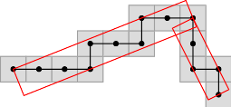
Arithmetic in DG: lattice polytopes/convex hulls
$P \subset \mathbb{R}^d$ is a lattice polytope with nonempty interior, then
$$f_k \ll c_n(Vol\,\,P)^\frac{d-1}{d+1}$$
In 2D, the largest lattice convex polygon in a $[1\ldots N]^2$ domain is such that
$$f_1 = \frac{12}{(4\pi^2)^{1/3}}N^{2/3} + O(N^{1/3}\log(N))$$
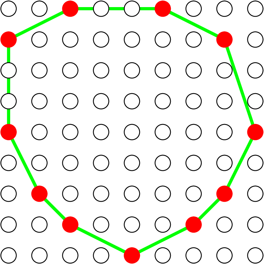
$\Rightarrow$ efficient output sensitive convex hull computation
Arithmetic in DG: geometry on bounded lattices
Given $n$ points in the plane in a $[0\ldots U]^2$ domain ($U\leq 2^m$), then expected time for Voronoi diagram / Delaunay triangulation is $$O\left (\min\left\{ n\log n, n\sqrt{\log U}\right \}\right)$$ (unit cost RAM with word size $m$)
- Radix-sort trick
- Special data structure Van Emde Boas tree
- ...
Separable volumetric transformation
 |

|

|

|
|

|

|

|
Separable and efficient algorithms for Distance transformation, Voronoi map, Reverse distance transformation, Power map, Medial Axis extraction... and for a large class of norms.
[Hirata, Breu et al., C. ...]
Rigid motions on discrete spaces
 [Kacper Pluta]
Computational homology applied to discrete objects
 [Aldo Gonzalez Lorenzo]
Few applications
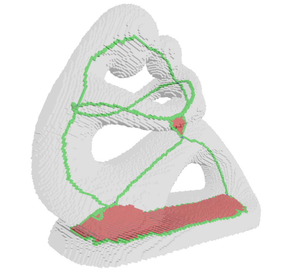
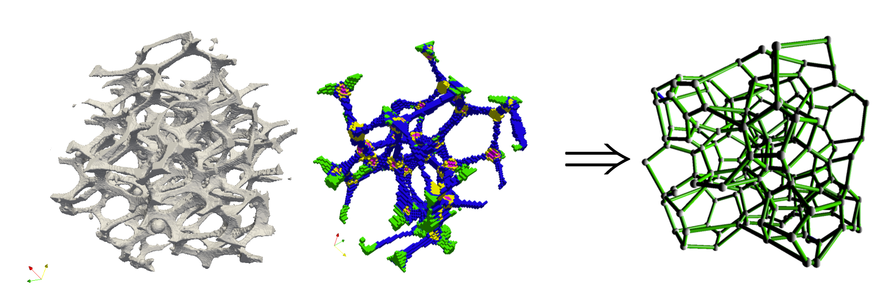
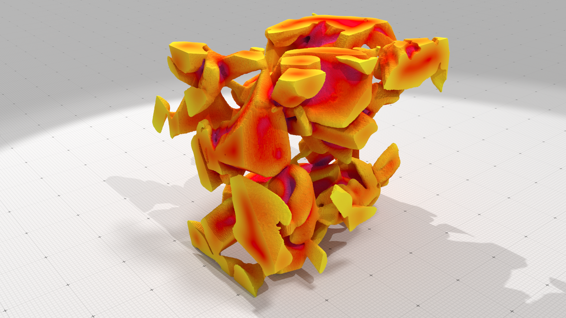
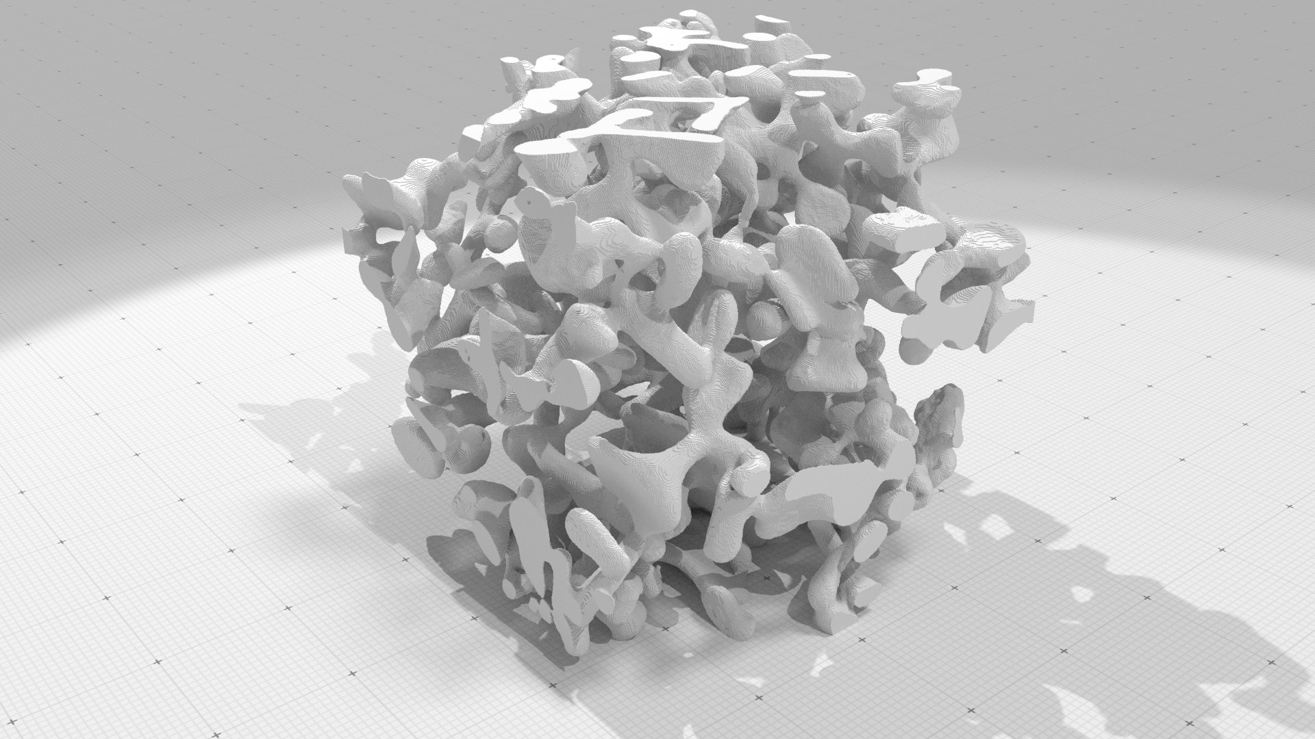
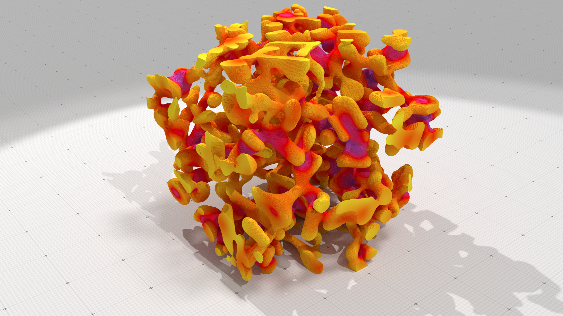
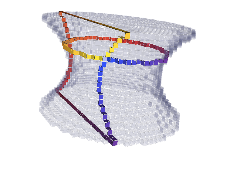
Application example: metallic foam characterizationdigitalFoam
Plastic/metallic foam topological and geometrical analysis and correlation to foam efficiency in catalytic reactors
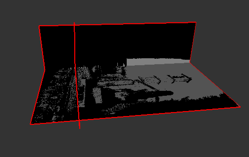
Micro-tomographic images $\rightarrow$ binary digital object $\rightarrow$ graph reconstruction with metric properties
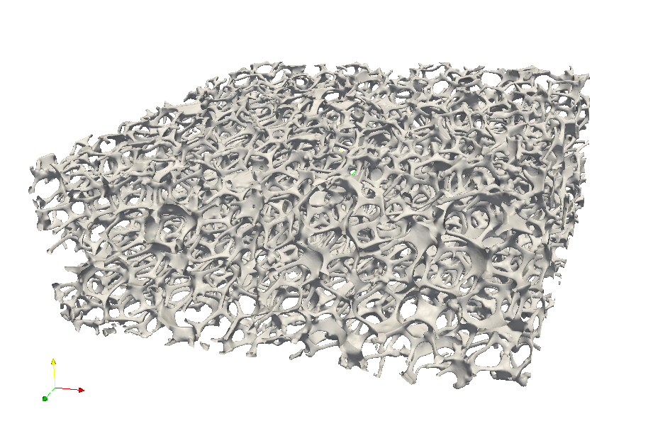
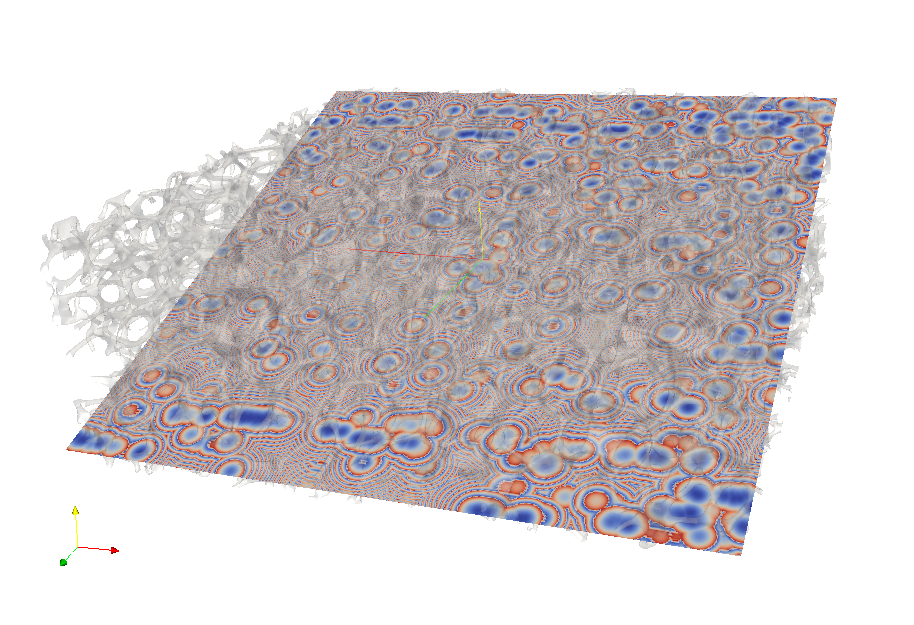
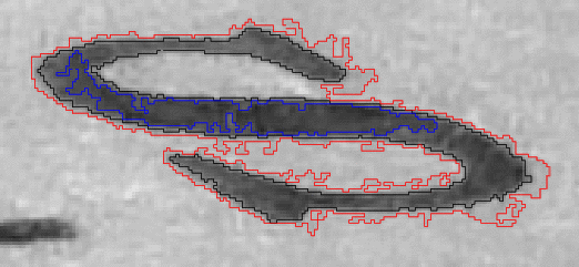
Application: digital snow metamorphism digitalSnow 
(LIRIS, LAMA, CNRM/CEN MétéoFrance)
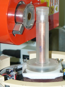
3SR Lab and CEN/CNRM - GAME URA 1357/Météo-France - CNRS
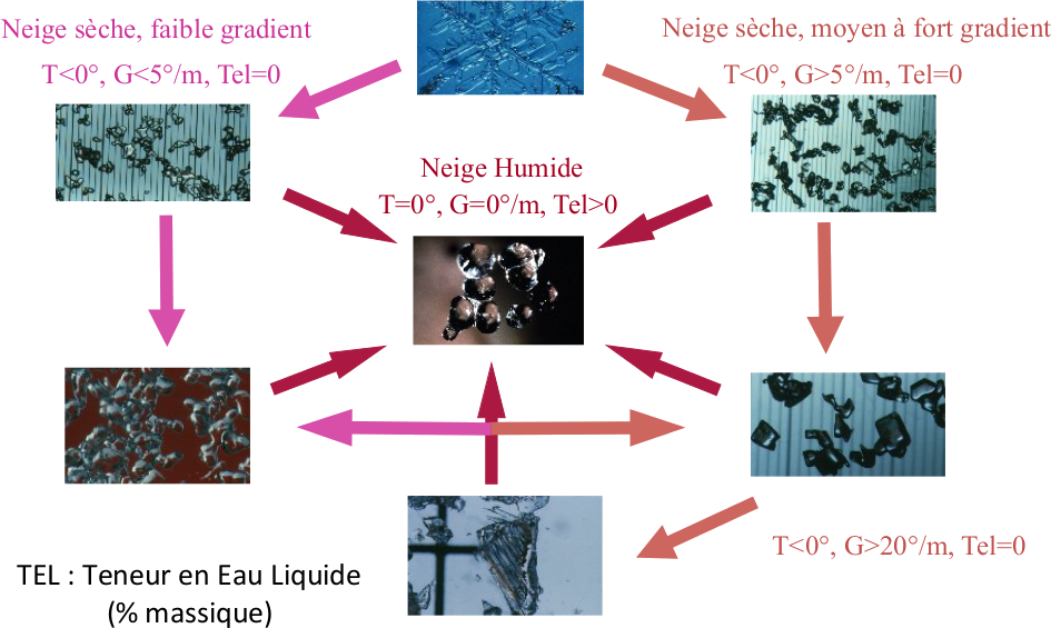
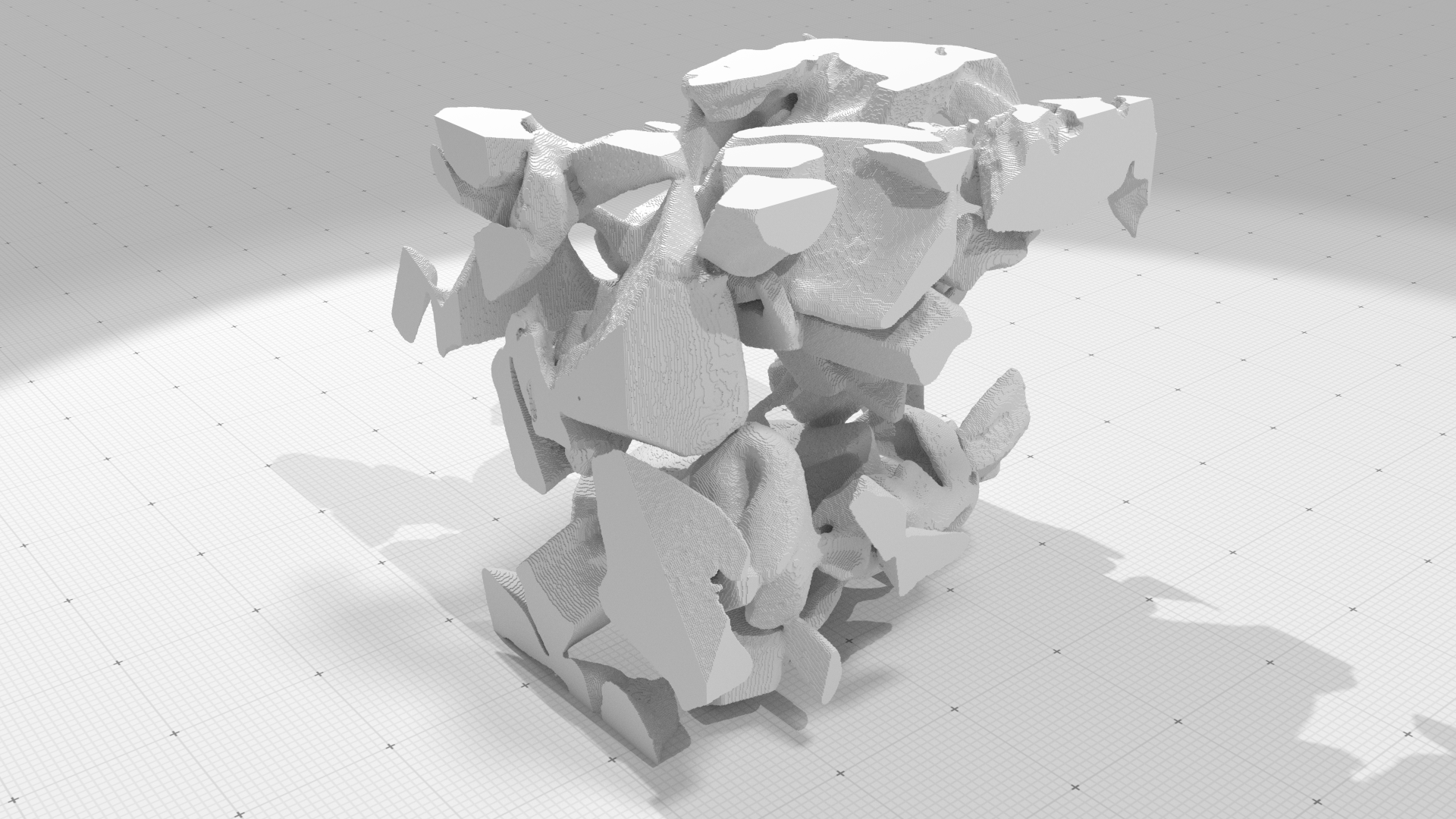
- Volumetric analysis (thickness quantification...)
- Curvature tensor estimation at ice/air interface
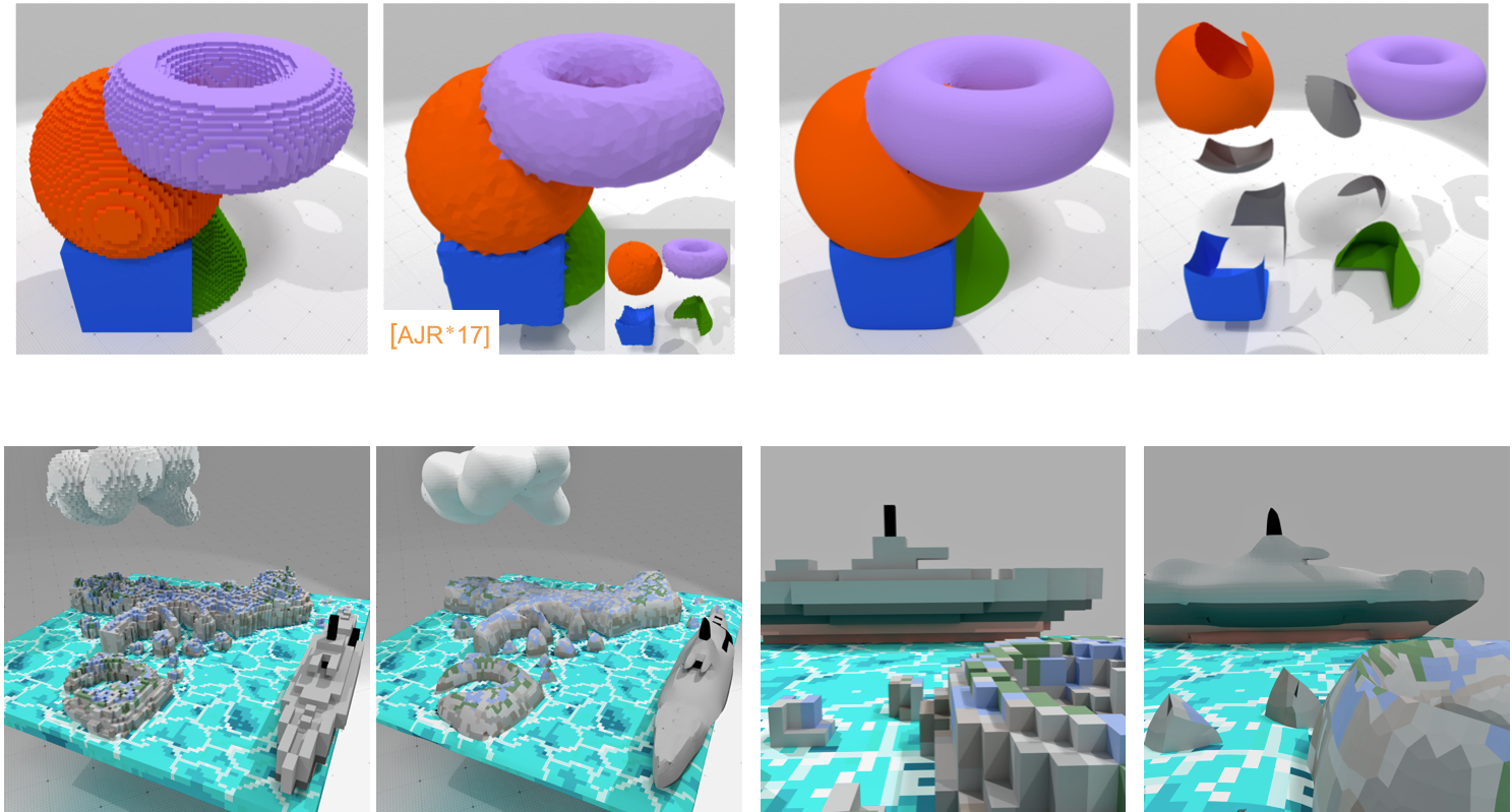
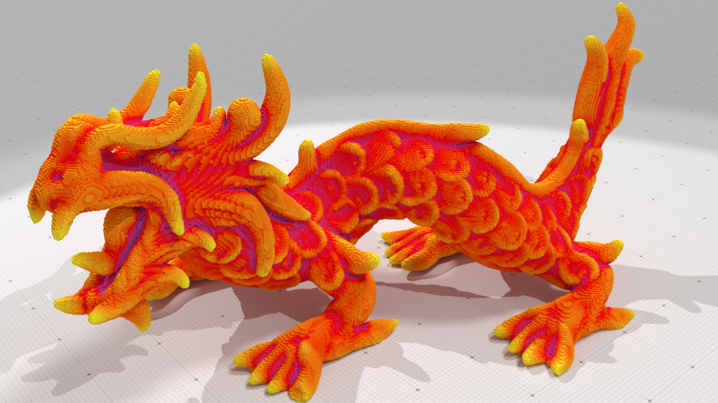
Digital Geometry in Computer Graphics
Digital Geometry in Computer Graphics
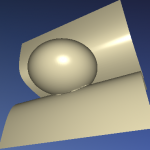
- Trivial CSG operators
- Efficient geometrical proxy data-structures for modeling
- Participating media modeling
- Fluid simulation
- Multi-phase materials
- Many voxel based global illumination techniques
- ...
Tech
| |
| |
|
Tech
| |
| |
 |
Controllable Shape Synthesis for Digital Fabrication
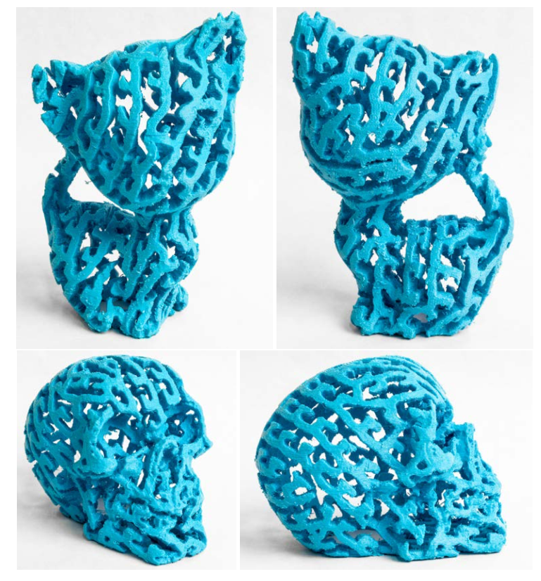 [Jérémie Dumas]
- Many input data are digital, let's deal with them!
- Trivial/easy topological representation of objects
- Very efficient data structures
- Great modeling tool for complex volumetric world!
- Exploit integer based representation:
- Consistent mathematical framework
- Exact geometrical predicates
- Arithmetical properties to speed the computations or the object characterization
- Exploit the regularity of the grid structure
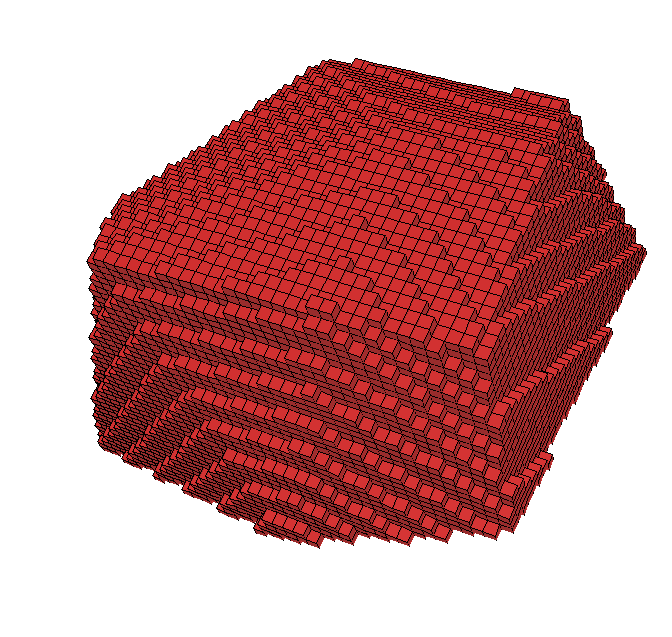
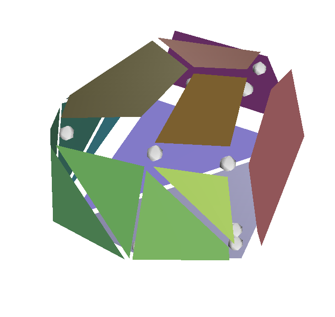
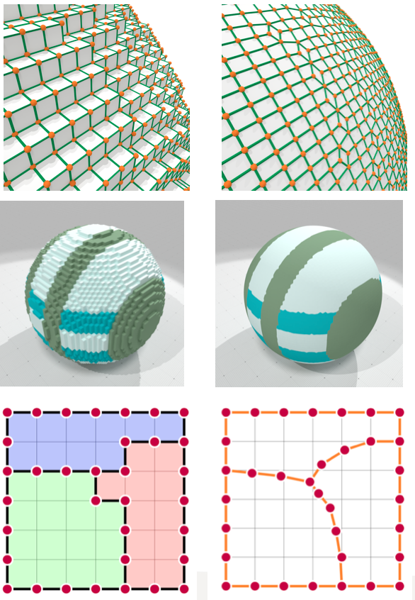
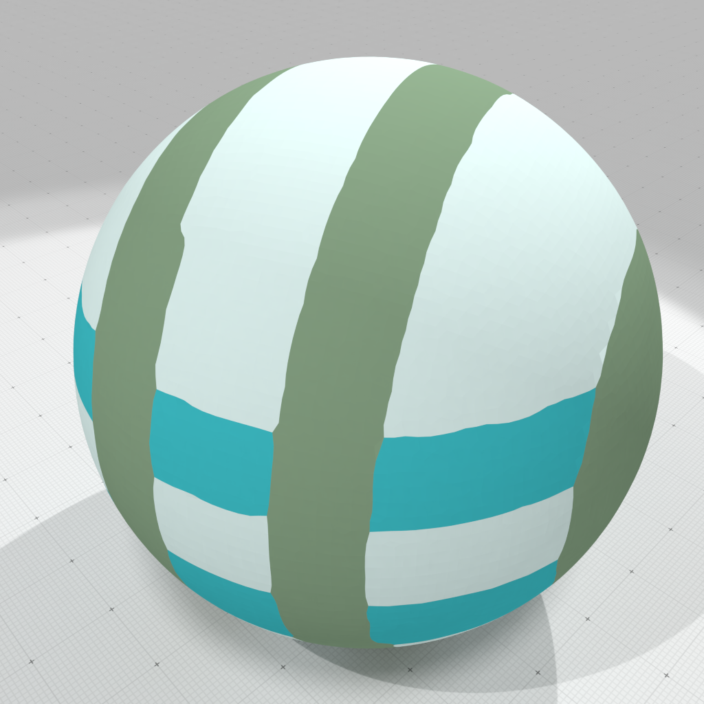
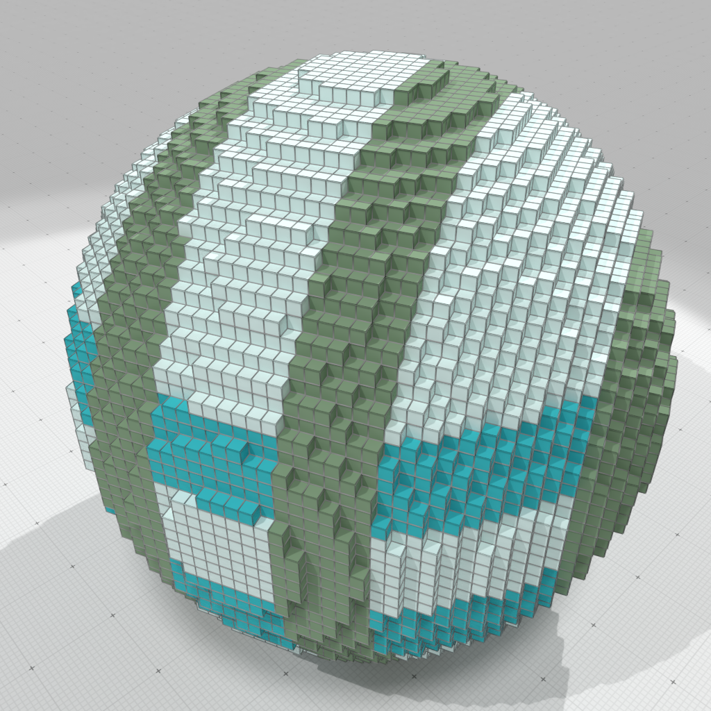
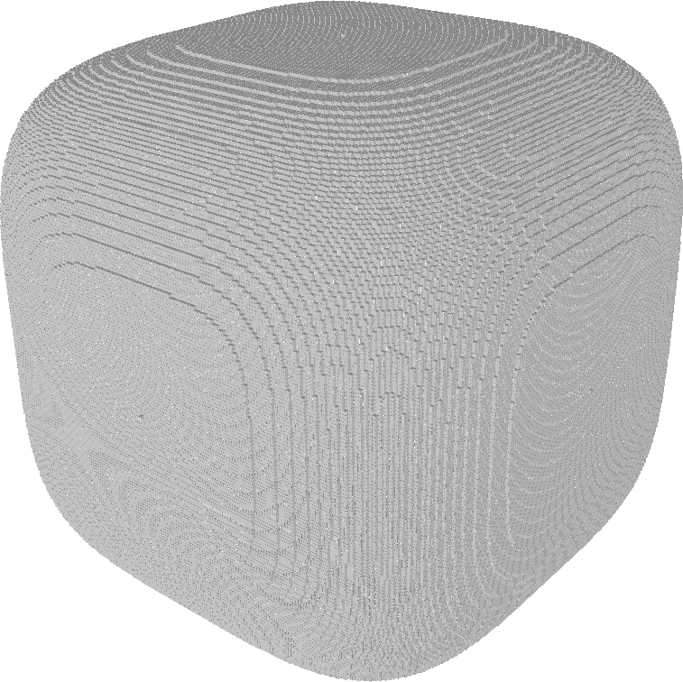
Example: Digital Surface Regularization
(with P. Gueth, J.-O. Lachaud)
Objectives
 |
|
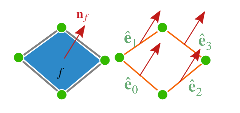
Input: consistent normal vector field $\{\mathbf{n}_{f}\}$
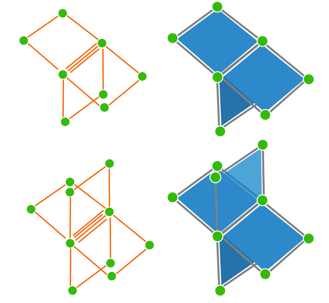
Variational apprach
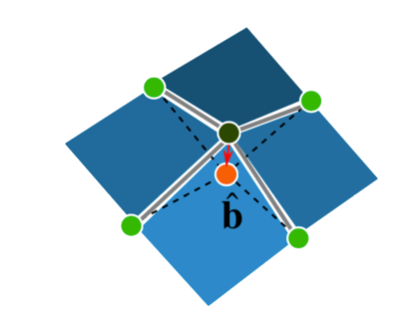
$\mathbf{p}_i$: vertices of the input digital surface, $\mathbf{n}_f$: normal vector per face
$\hat{\mathbf{p}}_i$: regularized vertices, $\hat{\mathbf{e}}_j$: edge between two regularized vertices, $\hat{\mathbf{b}}_i$: barycenter of the four adjacent regularized vertices of $\hat{\mathbf{p}}_i$ vertices
Variational apprach
$\mathbf{p}_i$: vertices of the input digital surface, $\mathbf{n}_f$: normal vector per face
$\hat{\mathbf{p}}_i$: regularized vertices, $\hat{\mathbf{e}}_j$: edge between two regularized vertices, $\hat{\mathbf{b}}_i$: barycenter of the four adjacent regularized vertices of $\hat{\mathbf{p}}_i$ vertices
Data attachment
Variational apprach
$\mathbf{p}_i$: vertices of the input digital surface, $\mathbf{n}_f$: normal vector per face
$\hat{\mathbf{p}}_i$: regularized vertices, $\hat{\mathbf{e}}_j$: edge between two regularized vertices, $\hat{\mathbf{b}}_i$: barycenter of the four adjacent regularized vertices of $\hat{\mathbf{p}}_i$ vertices
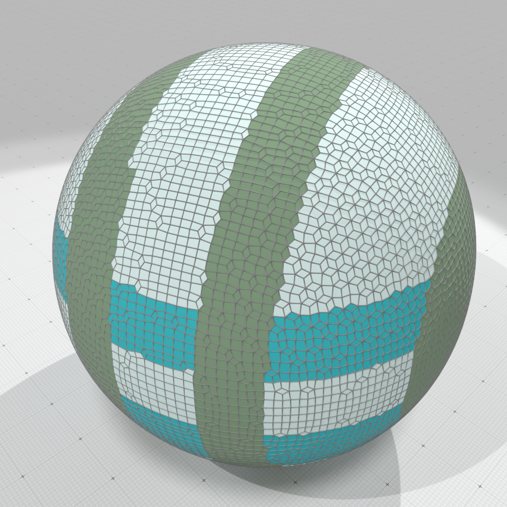
Data attachment + Quad alignement
Variational apprach
$\mathbf{p}_i$: vertices of the input digital surface, $\mathbf{n}_f$: normal vector per face
$\hat{\mathbf{p}}_i$: regularized vertices, $\hat{\mathbf{e}}_j$: edge between two regularized vertices, $\hat{\mathbf{b}}_i$: barycenter of the four adjacent regularized vertices of $\hat{\mathbf{p}}_i$ vertices
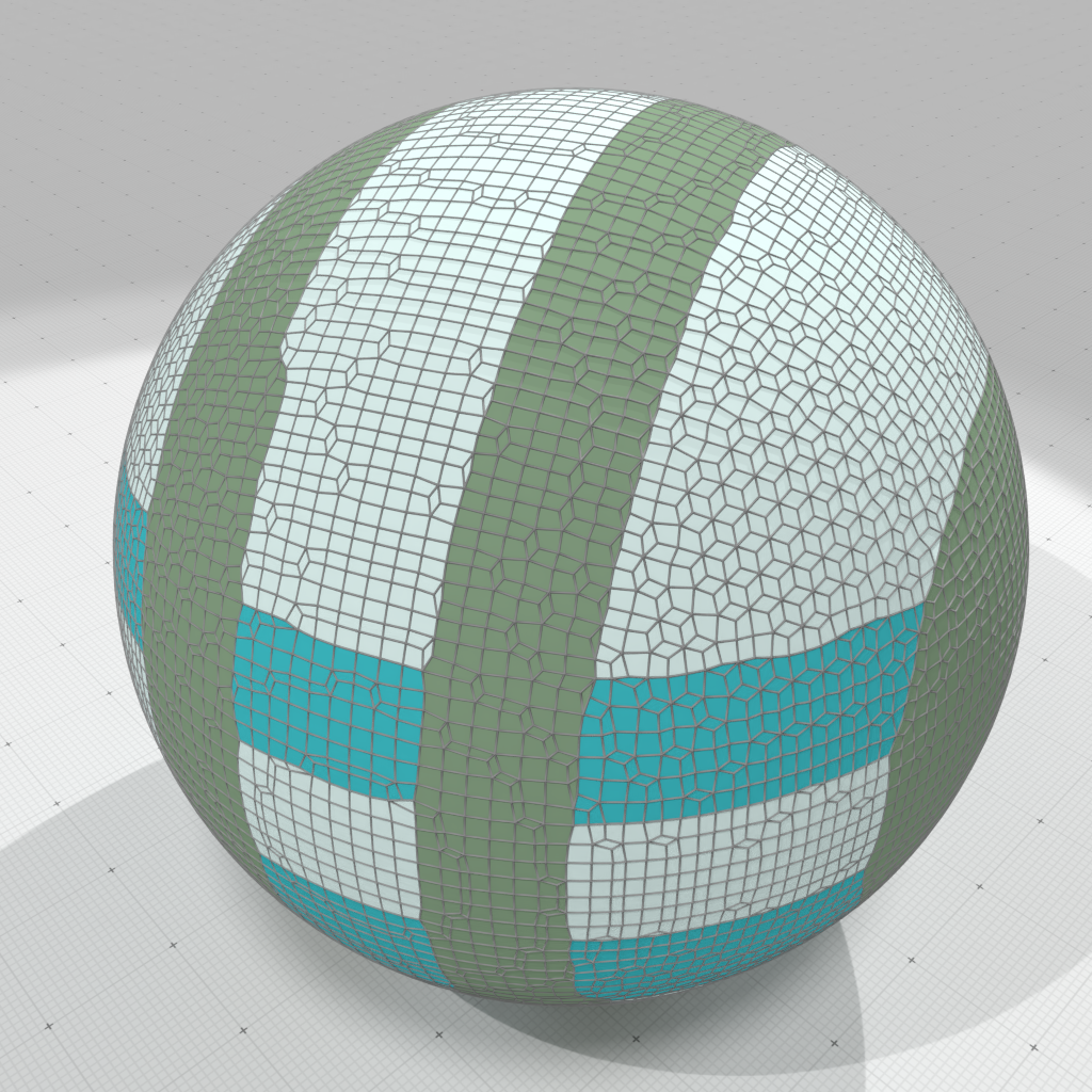
Data attachment + Quad alignement + Fairness term
Minimizing the energy
$\Rightarrow$ Optimal position given by solving a linear system
$\Rightarrow$ Efficient interactive regularization on GPU 😀
Multilabel case
$\Rightarrow$ Same formulation and trivial regularization thanks to the grid structure
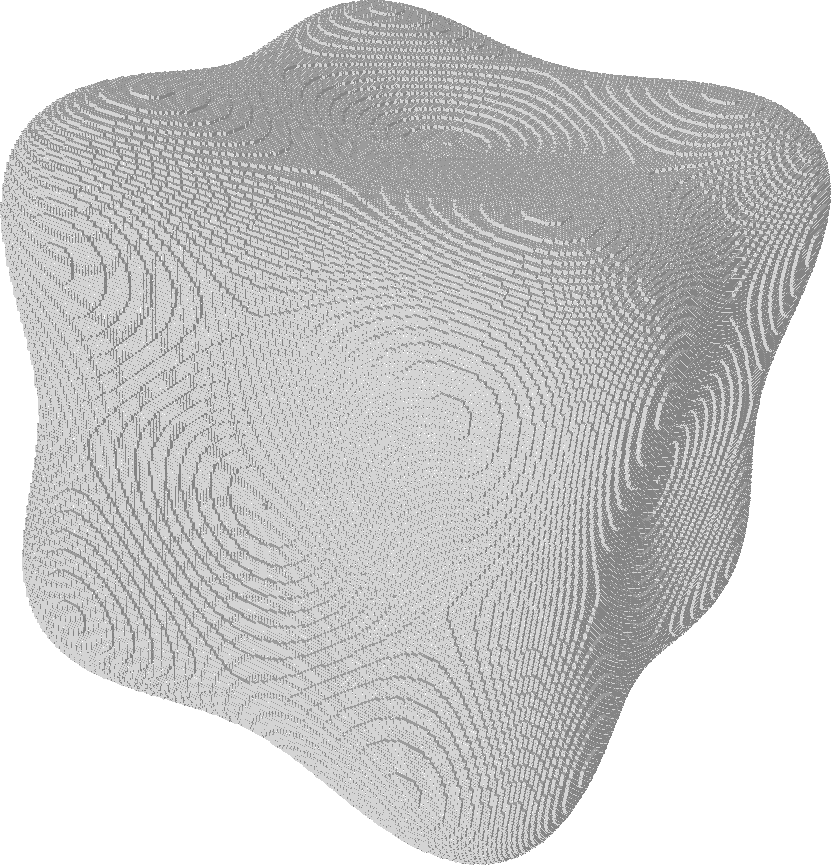
Tweaking the fairness term
 |
 |
 |
 |
 |
 |
Digital Geometry point of view: theoretical guarantees
If $M$ is smooth (positive reach) and $M_h:=M\cap ( h\cdot\mathbb{Z}^3)$ its digitization on a grid with gridstep $h$, then $$ \frac{1}{n}\sum_{i=1}^{n} \|\mathbf{p}^*_i - \mathbf{p}_i\| \leq C\cdot h \quad\quad \frac{1}{n}\sum_{i=1}^{n}\,d(\mathbf{p}^*_i, \partial M) \leq C'\cdot h$$
If normal vectors $\{\mathbf{n}_ƒ\}$ are multigrid convergent, normal vectors to regularized quads are also multigrid convergent and we have an even better approximation of $\partial M$
euh..."Multigrid convergent vector field ?" 🤔
Geometrical inference: multigrid convergence of curvature tensor
(with J. Levallois, J.-O. Lachaud)
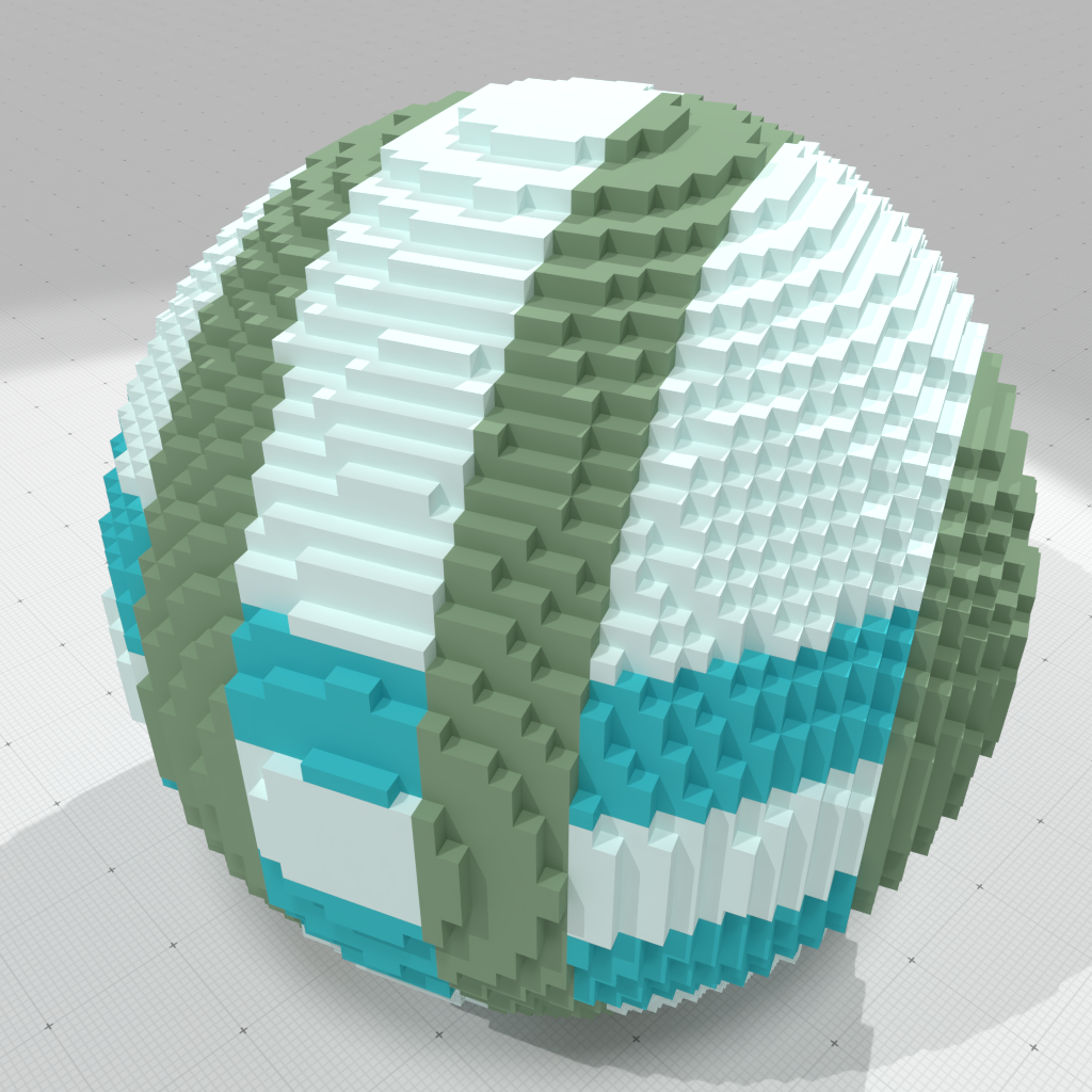
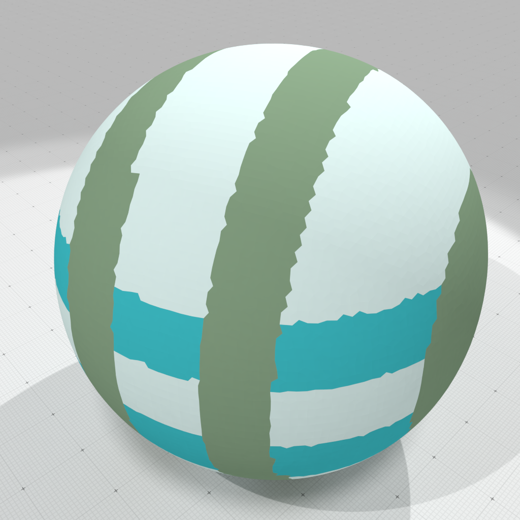
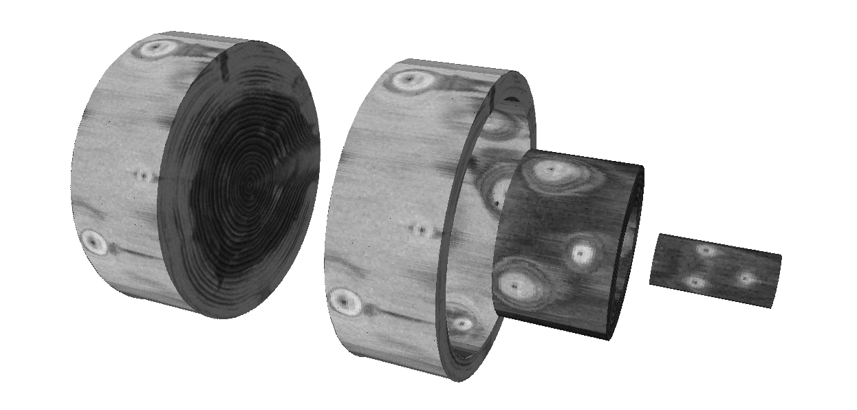
Digitization model
Given $\Shape \subset \R^d$, its digitization at gridstep $h$ is $$\DigF{\Shape}{h} = \left(\frac{1}{h} \cdot \Shape\right) \cap \Z^d$$
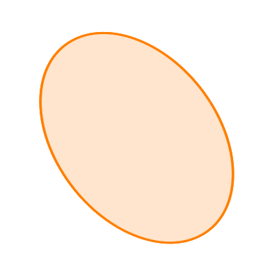
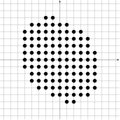
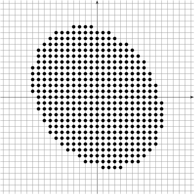
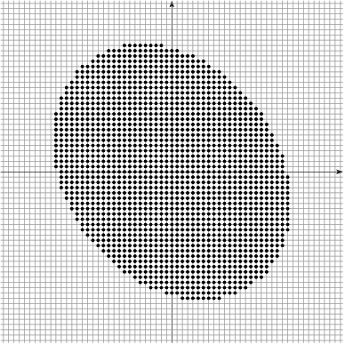
Example: $|\DigF{\Shape}{h}|$ converges to the area of $\Shape$ as $h\rightarrow 0$
[Gauss, Dirichlet, Huxley...]
Multigrid Convergence of a local estimator
Given a digitization process $\AnyDig$, a local discrete geometric
estimator $\hat{E}$ of some geometric quantity $E$ is multigrid
convergent for the family of shapes $\Shapes$ if and only if, for any $\Shape
\in \Shapes$, there exists a grid step $h_\Shape>0$ such that the
estimate $\hat{E}(\AnyDig_{\Shape}(h),\hat{\vx},h)$ is defined for all
$\hat{\vx} \in \Bd{\Body{\AnyDig_{\Shape}(h)}{h}}$ with $0< h< h_\Shape$, and for
any $\vx \in \dS$,
$$
\forall \hat{\vx} \in \Bd{\Body{\AnyDig_{\Shape}(h)}{h}} \text{ with } \| \hat{\vx} -\vx\|_\infty
\le h, \\ \quad\quad \color{myred}{|
\hat{E}(\AnyDig_{\Shape}(h),\hat{\vx},h) - E(\Shape,\vx) | \le \tau_{\Shape,\vx}(h)},
$$
where $\tau_{\Shape,\vx}: \R^{+} \setminus\{0\} \rightarrow \R^+$ has null limit at
$0$. The convergence is uniform for
$\Shape$ when every $\tau_{\Shape,\vx}$ is bounded from above by a function
$\tau_\Shape$ independent of $\vx \in \Bd{\Shape}$ with null limit at $0$.
- $|\DigF{\Shape}{h}|$ is multigrid convergence with convergence speed in $O(h)$ for convex shapes [Gauss, Dirichlet]
- $|\DigF{\Shape}{h}|$ is multigrid convergence with convergence speed in $O(h^{\frac{15}{11}+\epsilon})$ for shapes with strictly $C^3$-convex boundaries [Huxley]
- Geometrical moments ✓
- Length, surface area ✓
- Tangent, normal vectors ✓
Digital/Continuous mapping

- The Hausdorff between $\partial \Shape$ and $\partial_h\Shape$ is bounded by $\sqrt{d}h/2$
- For $d=2$, there exists an homeomorphism between $\partial X$ and $\partial_h X$
- For $d\geq 3$, no homeomorphism ☹, but
- Projection operator $\xi:\,\partial_h\Shape\rightarrow\partial \Shape$ is surjective
- Area of non-injective parts of $\xi$ the tends to zero
- $\Rightarrow$ Great for integration🙂
Digitization as an Hausdorff sampling of the continuous object

Can we estimate the curvature tensor on digital surfaces with multigrid convergence properties ?
Related works (selection)
- Meshes
- Local estimators (1- ou 2-rings) [Surazhsky et al. 2003][Gatzke, Grimm 2006]
- Gauss-Bonnet formula based estimators [Xu 2006]
- Normal cycles [Cohen-Steiner, Morvan 2006]
- Point Clouds
- Jet-Fitting approaches [Cazals, Pouget 2005]
- Voronoi cell covariance measure (VCM) [Alliez et al. 2007][Merigot et al. 2011][Cuel et al. 2014]
→ precision depends on the mesh/point cloud quality
→ incompatible constraints on convergence theorem w.r.t. digital surface
- Digital surfaces
- From digital object recognition in 2D (Segments, Arcs) [Coeurjolly et al. 2001][Roussillon et al. 2011]
- Binomial Convolution based approaches [Malgouyres et al. 2008][Esbellin et al. 2011]
- Polynomial fitting [Provot, Gérard 2014]
Generic approach: Varifold theory [Buet 2014][Buet et al. 2015]
Main contributions
| Quantity | 2D/3D | Parameter | Theoretical convergence | Experimental convergence |
|---|---|---|---|---|
$\CurvH{R}$ |
2D | $R$ |
$O\left(h^\frac{1}{3}\right)$ when $R=kh^\frac{1}{3}$ | $O\left(h^\frac{1}{3}\right)$ when $R=kh^\frac{1}{3}$ |
$\MeanCurvH{R}$ |
3D | $R$ |
$O\left(h^\frac{1}{3}\right)$ when $R=kh^\frac{1}{3}$ | $O\left(h^\frac{1}{3}\right)$ when $R=kh^\frac{1}{3}$ |
$\PrincCurvH{i}{R}$ |
3D | $R$ |
$O\left(h^\frac{1}{3}\right)$ when $R=kh^\frac{1}{3}$ | $O\left(h^\frac{1}{3}\right)$ when $R=kh^\frac{1}{3}$ |
$\CurvHS$ |
2D | no |
$O\left(h^\frac{1}{3} \log^2(h)\right)$ |
$O\left(h^\frac{1}{3}\right)$ |
$\MeanCurvHS$ |
3D | no |
* |
$O\left(h^\frac{1}{3}\right)$ |
$\PrincCurvHS{i}$ |
3D | no |
* |
$O\left(h^\frac{1}{3}\right)$ |
Integral Invariant approach (in 2D)

$${\color{mydarkred}A_R(\Shape,\vx)} \EqDef \int_{\Ball{R}{\vx}} \chi(\vp)d\vp$$
Taylor expansion of local smooth surface patch ($\Shapes^{2-SC}$) :
\[
\tilde{\kappa}^{R}(\Shape,\vx) \EqDef \frac{3\pi}{2{{R}}} - \frac{3 {\color{mydarkred}A_R(\Shape,\vx)}}{{{R}}^3}
\]
$\quad \CurvT{R}(\Shape,\vx) = \Curv(\Shape,\vx) + {\color{mydarkred}O(R)} $
$R \rightarrow 0$ does not make sense on digital structures
Overall proof scheme
→ $A_R(\Shape,\vx) \rightarrow \AreaC(\Ball{R/h}{\vx/h} \cap \DigF{\Shape}{h})$
+ [Pottmann et al. 2007] $\quad\CurvH{R}(\DSh,\vx,h)$
→ $\CurvH{R}(\DSh,\hat{\vx},h) \rightarrow \Curv(\Shape,\vx)$
Area estimator "à la" Gauss
\[ {\color{myblue}\AreaC(\DSh)} \EqDef h^2 \Card (\DSh) \]
$\quad \AreaC(Y) = \Area(\Shape) + {\color{myblue}O(h^\beta)}\quad\quad\text{with}\quad \beta \ge 1$
- $\beta = 1$ for $\Shapes^C$ [Gauss, Dirichlet]
- $\beta = \frac{15}{11}-\epsilon$ for $\Shapes^{3-SC}$ (non null curvature) [Huxley 1990]
Area estimator "à la" Gauss
\[ {\color{myblue}\AreaC(Y)} \EqDef h^2 \Card (Y) \quad\quad\text{with}\quad Y = \Ball{R/h}{\vx/h} \cap \DigF{\Shape}{h} \]
$\quad \AreaC(Y) = A_R(\Shape,\vx) + {\color{myblue}O(h^\beta R^{2-\beta})} \quad\quad\text{with}\quad \beta \ge 1$


Overall proof scheme - 1/3
→ $A_R(\Shape,\vx) \rightarrow \AreaC(\Ball{R/h}{\vx/h} \cap \DigF{\Shape}{h})$

+ [Pottmann et al. 2007] $\quad\CurvH{R}(\DSh,\vx,h)$
→ $\CurvH{R}(\DSh,\hat{\vx},h) \rightarrow \Curv(\Shape,\vx)$
Curvature estimation by digital integration
\[ \hat{\kappa}^{R}(\DigF{\Shape}{h},\vx,h) \EqDef \frac{3\pi}{2{{R}}} - \frac{3 {\color{myblue}\AreaC(Y)}}{{{R}}^3} {\color{mydarkred}+O(R)} \quad\text{with}\quad Y = \Ball{R/h}{\vx/h} \cap \DigF{\Shape}{h} \]
Overall proof scheme - 2/3
→ $A_R(\Shape,\vx) \rightarrow \AreaC(\Ball{R/h}{\vx/h} \cap \DigF{\Shape}{h})$
+ [Pottmann et al. 2007] $\quad\CurvH{R}(\DSh,\vx,h)$
→ $\CurvH{R}(\DSh,\hat{\vx},h) \rightarrow \Curv(\Shape,\vx)$
Positioning Error

― $\pi^\Shape_h(\hat{\vx})$

Overall proof scheme - 3/3
→ $A_R(\Shape,\vx) \rightarrow \AreaC(\Ball{R/h}{\vx/h} \cap \DigF{\Shape}{h})$
+ [Pottmann et al. 2007] $\quad\CurvH{R}(\DSh,\vx,h)$
→ $\CurvH{R}(\DSh,\hat{\vx},h) \rightarrow \Curv(\Shape,\vx)$
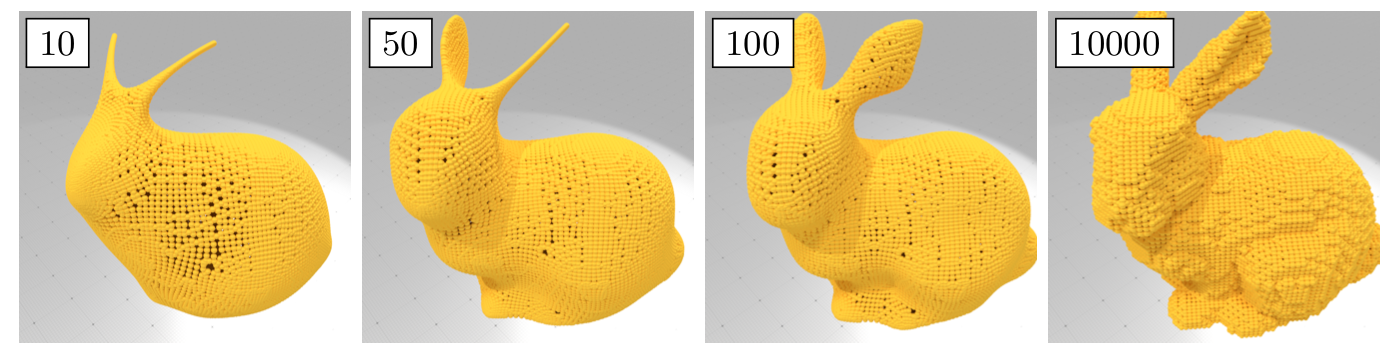
Multigrid convergence of the digital curvature estimator
→ Setting $R=kh^\alpha$, we select $\alpha$ to minimize all errors.
Mean curvature on digital surfaces

Let $\Shape$ be a convex shape in $\R^3$ with $C^3$ bounded positive curvature boundary.
$ Y = \Ball{R/h}{\vx/h} \cap \DigF{\Shape}{h} $
$ {\color{myblue}\VolC(Y)} \EqDef h^3 \Card (Y) $
$ \MeanCurvH{R}(\DigF{\Shape}{h},\vx,h) \EqDef \frac{8}{3{{R}}} - \frac{4 {\color{myblue}\VolC(Y)}}{\pi R^4} $
Principal curvature on digital surfaces
Let $\Shape$ be a convex shape in $\R^3$ with $C^3$ bounded positive curvature boundary.
$Y = \Ball{R/h}{\vx/h} \cap \DigF{\Shape}{h}$
${\color{myblue}\DMom{pqs}{h}(Y)} \EqDef h^{3+p+q+s} \sum y_1^{p} y_2^{r} y_3^{s}$
\[ {\color{myblue}\DCov{h}(Y)} \EqDef \left\lbrack{\color{myblue} \begin{array}{ccc} \DMom{200}{h}(Y) & \DMom{110}{h}(Y) & \DMom{101}{h}(Y)\\ \DMom{110}{h}(Y) & \DMom{020}{h}(Y) & \DMom{011}{h}(Y)\\ \DMom{101}{h}(Y) & \DMom{011}{h}(Y) & \DMom{002}{h}(Y) \end{array}} \right\rbrack - \frac{1}{\color{myblue}\DMom{000}{h}(Y)} \left\lbrack{\color{myblue} \begin{array}{c} \DMom{100}{h}(Y) \\ \DMom{010}{h}(Y) \\ \DMom{001}{h}(Y) \\ \end{array}} \right\rbrack \otimes \left\lbrack{\color{myblue} \begin{array}{c} \DMom{100}{h}(Y) \\ \DMom{010}{h}(Y) \\ \DMom{001}{h}(Y) \\ \end{array}} \right\rbrack^T \]
Matrix perturbation theory (1/2)
Invariance by translation
- $\forall Y \subset \R^3, \forall \vv \in \R^3, \Cov(Y + \vv) = \Cov(Y)$
- $\forall Z \subset \Z^3, \forall \vv \in \Z^3, \DCov{h}(Z + \vv) = \DCov{h}(Z)$
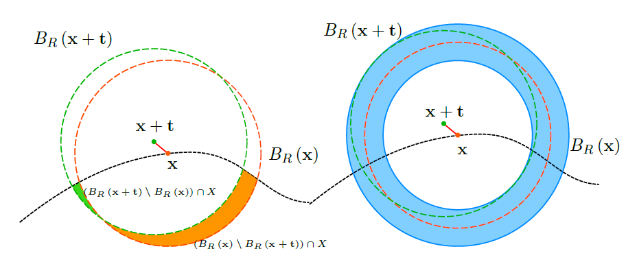
\[ \begin{align} \left| \Mom{000}(\Ball{R}{\vx + \vt} \cap \Shape) - \Mom{000}(\Ball{R}{\vx} \cap \Shape) \right| & \le O(t R^2), \label{eq:zero-moments-ball-position-error} \\ \left| \Mom{100}(\Ball{R}{\vx + \vt} \cap \Shape) - \Mom{100}(\Ball{R}{\vx} \cap \Shape) \right| & \le O(t R^3) + O( \|\vx\|_\infty t R^2 ), \label{eq:first-moments-ball-position-error}\\ \left| \Mom{200}(\Ball{R}{\vx + \vt} \cap \Shape) - \Mom{200}(\Ball{R}{\vx} \cap \Shape) \right| & \le O(t R^4) + O( \|\vx\|_\infty t R^3 ) + O( \|\vx\|^2_\infty t R^2 ). \label{eq:second-moments-ball-position-error} \end{align} \]
Matrix perturbation theory (2/2)
Let $\lambda_i(M)$ (resp. $\lambda_i(M')$) be the $i$-th eigenvalue of a symmetric matrix $M$ (resp. $M'$) with , then \[ \begin{equation} \max_{i}| \lambda_i(M) - \lambda_i(M')| \le \|M-M'\| \end{equation} \]
Principal curvature on digital surfaces
\[ \begin{align} &\PrincCurvH{1}{R}(\DSh,\vx,h) \EqDef \frac{6}{\pi R^6}\left({\color{myblue}\hat{\lambda}_2} - 3{\color{myblue}\hat{\lambda}_1}\right) + \frac{8}{5R}\\ &\PrincCurvH{2}{R}(\DSh,\vx,h) \EqDef \frac{6}{\pi R^6}\left({\color{myblue}\hat{\lambda}_1} - 3{\color{myblue}\hat{\lambda}_2}\right) + \frac{8}{5R}\\ &\PrincDirH{1}{R}(\DSh,\vx,h) \EqDef {\color{myblue}\hat{\nu}_1}\\ &\PrincDirH{2}{R}(\DSh,\vx,h) \EqDef {\color{myblue}\hat{\nu}_2}\\ &\NormalDirH{R}(\DSh,\vx,h) \EqDef {\color{myblue}\hat{\nu}_3} \end{align} \]
\[ \begin{align} &\exists h_\Shape \in \R^+,\,\, \forall h \in \R,\,\, 0 < h < h_\Shape,\,\, \,\,\nonumber\quad \quad\quad \quad\\ &\forall \vx \in \Bd{\Shape}, \quad \forall \hat{\vx} \in \Bd{\Body{\DSh}{h}} \text{ avec } \| \hat{\vx} -\vx\|_\infty \le h, \nonumber\quad \quad\quad \quad \\ &\quad \quad\quad \quad\| \PrincDirH{1}{R}( \DSh, \hat{\vx}, h ) - \PrincDir{1}(\Shape, \vx) \| \le \frac{1}{|\PrincCurv{1}(\Shape,\vx)-\PrincCurv{2}(\Shape,\vx)|} O(h^{\frac{1}{3}})\,, \\ &\quad \quad\quad \quad\| \PrincDirH{2}{R}( \DSh, \hat{\vx}, h ) - \PrincDir{2}(\Shape, \vx) \| \le \frac{1}{|\PrincCurv{1}(\Shape,\vx)-\PrincCurv{2}(\Shape,\vx)|} O(h^{\frac{1}{3}})\,, \\ &\quad \quad\quad \quad\| \NormalDirH{R}( \DSh, \hat{\vx}, h ) - \NormalDir(\Shape, \vx) \| \le O(h^{\frac{2}{3}})\,. \end{align} \]
Experimental validation design

| Shape | Quantity | Estimators |
|---|---|---|

|
$\CurvH{R}$ | MDCA, BC, MDSS |
|
$\MeanCurvH{R}$, $\PrincCurvH{1}{R}$, $\PrincCurvH{2}{R}$ | JetFitting |
Few results

In summary
- Robust
- Efficient implementation
- Parametrized by a integration radius $R$ or a grid step $h$
- Proof relies on digital/continuous relationships and geometrical moment estimation
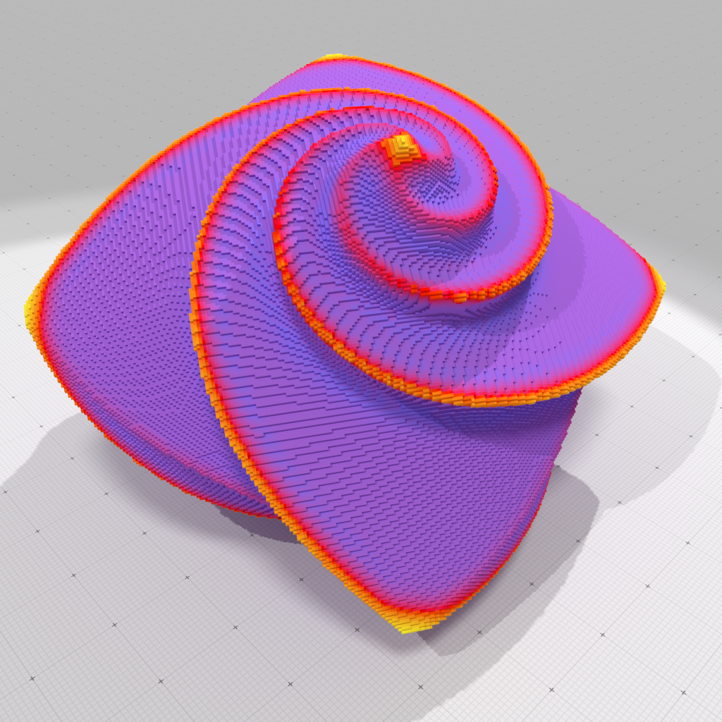
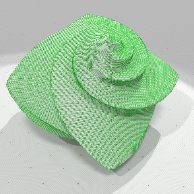
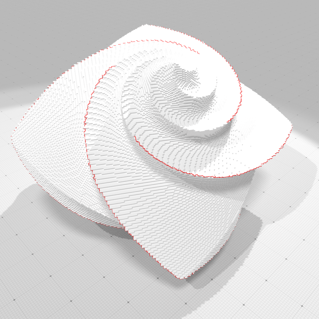
Piecewise smooth normal vector field 🤗
Piecewise smooth reconstruction of normal vector field on digital data
(with M. Foare, J.-O. Lachaud, P. Gueth)
Motivations
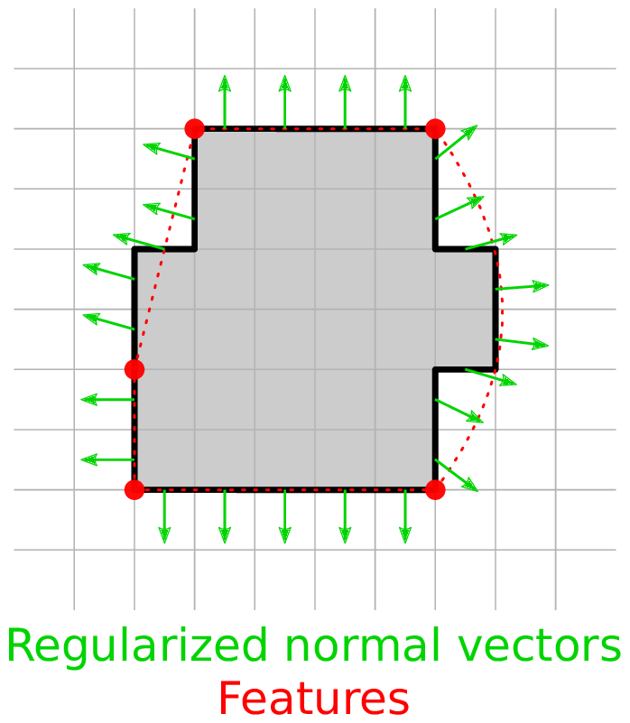
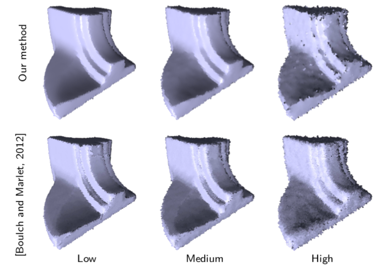
Anisotropic filtering the object surface normal vector field and feature extraction at the same time
|
|  |
|
|  |
$\Rightarrow$ None of them achieve both
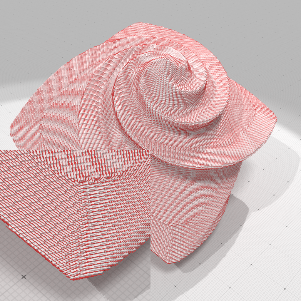
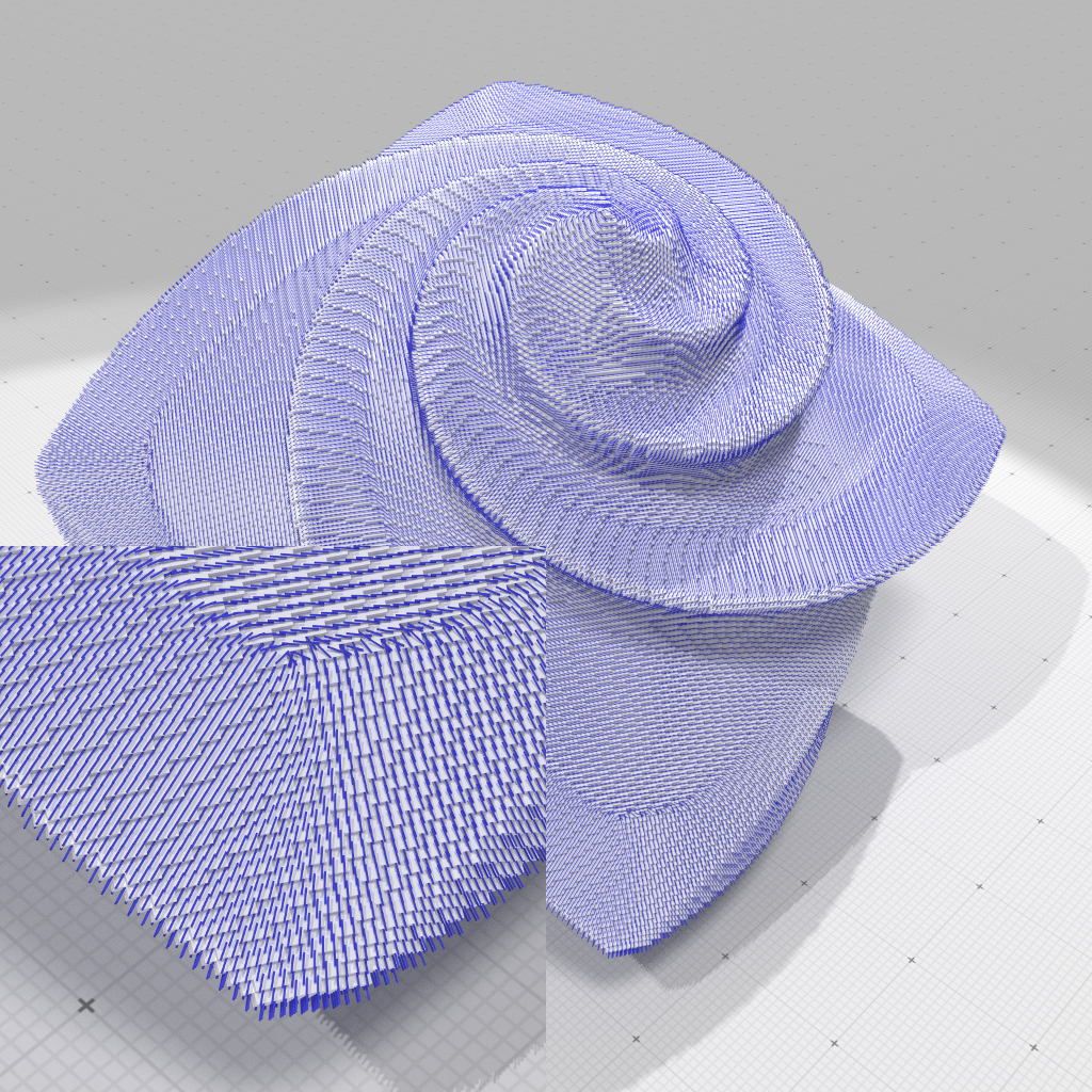
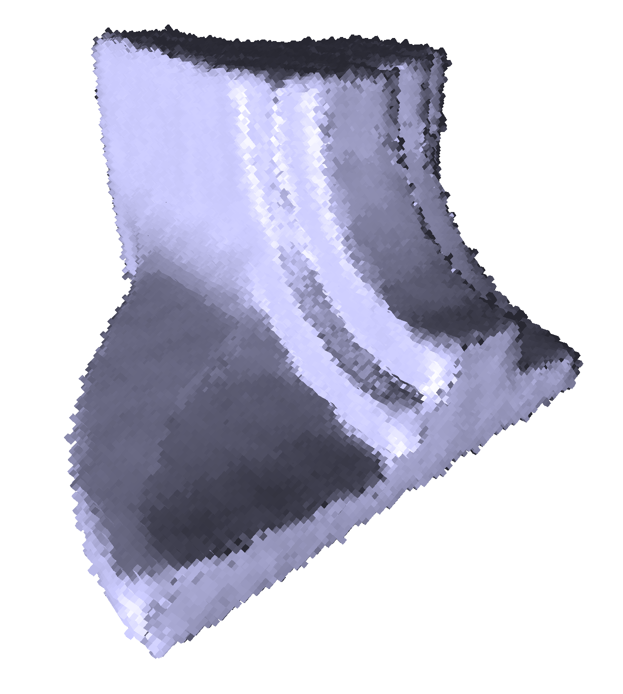
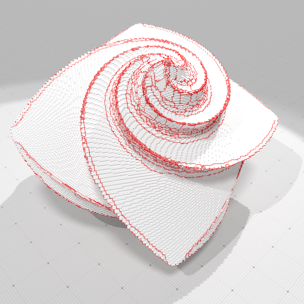
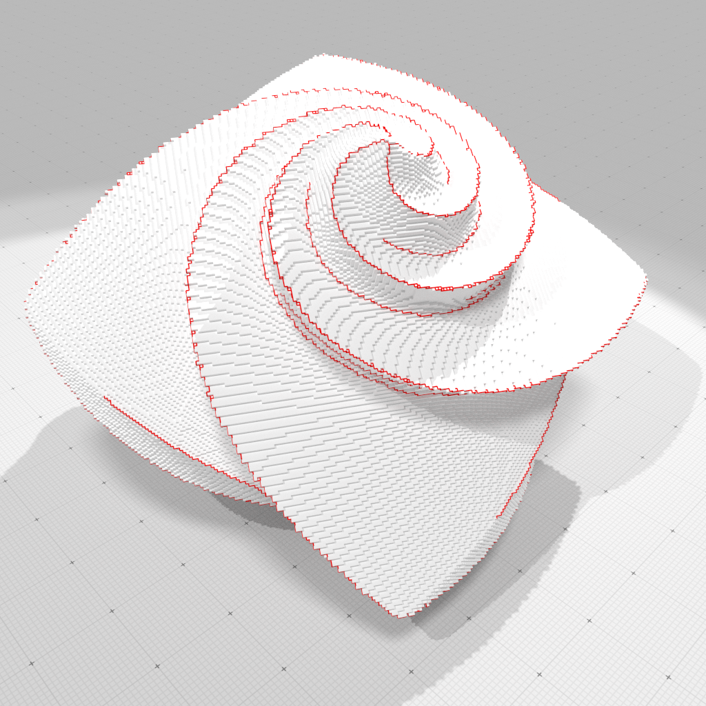
Method overview
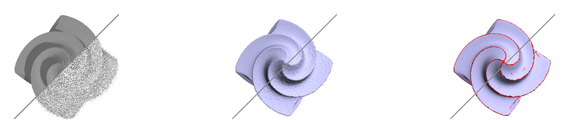
| Digital surface | Raw global normal vector field estimation | Piecewise regularized normal vector field + feature scalar field |
We want a (variational) formulation allowing us to control the smoothness of the reconstruction with respect of a given noise and the length of the discontinuities
$\Rightarrow$ we regularize an input normal vector field $g$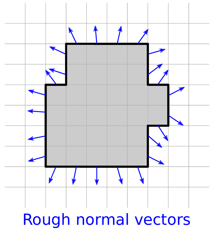
Mumford-Shah functional
$$\mathcal{MS} (K,u)= \underbrace{ \alpha \dint_{{M\backslash K}} | u - g |^2 \dx}_{\text{attachment term}} + \underbrace{\dint_{{M\backslash K}} | \grad u |^2 \dx}_{\text{smoothness term}} + {\underbrace{\lambda \hauss{1}(K \cap M)}_{\text{discontinuities length}}} $$
- $\mathcal{M}$ is the object surface
- ${g}$ is the input raw normal vector field
- ${u}$ is the regularized normal vector field
- ${K}$ is the discontinuities support set
- $\hauss{1}$ is the Hausdorff measure
But:
- Needs an explicit evaluation of $\hauss{1}(K\cap M)$
- We integrate over ${M\backslash K}$
- ${K}$ is to be optimized
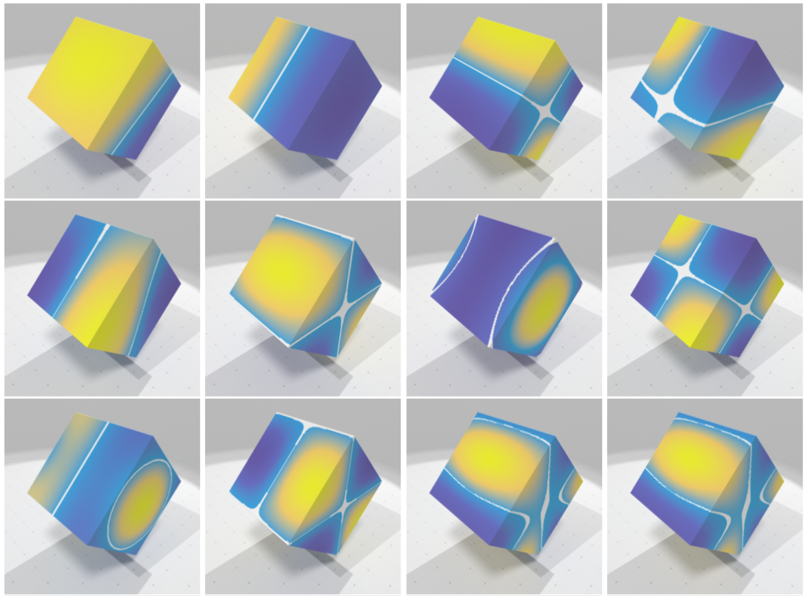
Ambrosio-Tortorelli functional
$$ \mathcal{AT}_\eps(u,v) = {\alpha} \underbrace{\dint_{{M}} |u - g|^{{2}} \dx}_{\text{attachment term}} + \underbrace{\dint_{{M}} |{v} \grad u|^{{2}} \dx}_{\text{smoothness term}} + \underbrace{{\lambda} \dint_{{M}} {\eps} |\grad {v}|^{{2}} + \frac{1}{4 {\eps}} |1 - {v}|^{{2}} \dx}_{\text{discontinuities length}}$$
- Two functions to optimize: $u$ (regularized normal vector field) and $v$ (feature scalar map, $\mathcal{M}\rightarrow [0,1]$)
- $v\approx 1$ on smooth parts, $v\approx 0$ near features
- Integration domain does not change
- No Hausdorff measure
- Quadratic terms
- the AT functional $\Gamma-$converges to Mumford-Shah's functional $\mathcal{AT}_\eps \gammaconv{\eps \to 0} \mathcal{MS}$
Ambrosio-Tortorelli functional
$$ \mathcal{AT}_\eps(u,v) = {\alpha} \underbrace{\dint_{{M}} |u - g|^{{2}} \dx}_{\text{attachment term}} + \underbrace{\dint_{{M}} |{v} \grad u|^{{2}} \dx}_{\text{smoothness term}} + \underbrace{{\lambda} \dint_{{M}} {\eps} |\grad {v}|^{{2}} + \frac{1}{4 {\eps}} |1 - {v}|^{{2}} \dx}_{\text{discontinuities length}}$$
- $\eps$ -- thickness of the feature set ($[distance]$)
- ${\alpha}$ -- attachment coefficient to control the smoothing strength ($[area^{-1}]$)
- $\lambda$ -- proportional to the length of discontinuities ($[distance^{-1}]$)
Discretization
"à la" Discrete Exterior Calculus [Hirani, Desbrun, Grady...]:
$\mathcal{M}$ is a cellular complex ($\mathcal{M}'$ its dual), $\sigma^k$ are $k-$cells of $\mathcal{M}$ (resp. $\sigma'^k$ of $\mathcal{M}'$)


- $k-$forms are vectors of $|\{\sigma^k\}|$ scalars
- Linear operators are matrices
- e.g.
- $d_k$ (exterior derivative) maps primal $k-$forms to primal $(k+1)-$forms
- wedge product $\alpha\wedge \beta$ maps $k-$forms and $l-$forms to $(k+l)-$forms
- Hodge-star $\star_k$ operator to maps primal $k-$forms to dual $k-$forms
- ...
Discretization (bis)
$$ \mathcal{AT}_\eps(u,v) = {\alpha} \underbrace{\dint_{{M}} |u - g|^{{2}} \dx}_{\text{attachment term}} + \underbrace{\dint_{{M}} |{v} \grad u|^{{2}} \dx}_{\text{smoothness term}} + \underbrace{{\lambda} \dint_{{M}} {\eps} |\grad {v}|^{{2}} + \frac{1}{4 {\eps}} |1 - {v}|^{{2}} \dx}_{\text{discontinuities length}}$$
$v$ is a primal $0$-form, $u$ is a triple of dual $0$-forms $(u_1,u_2,u_3)$ and we discretize $\mathcal{AT}_\epsilon$
$$\mathcal{AT}^d_\epsilon(u,v) \EqDef \alpha \sum_{i=1}^{3} \langle{u_i - g_i},{u_i - g_i}\rangle_\bar{0} + \sum_{i=1}^{3} \langle{v \wedge d_\bar{0} u_i},{v \wedge d_\bar{0} u_i}_\bar{1}\rangle_\bar{1} \\ \quad\quad\quad\quad\quad\quad+ \lambda \epsilon \langle{ d_{0} v },{ d_{0} v }\rangle_1 + \frac{\lambda}{4\epsilon} \langle{1 - v},{1 - v}\rangle_0$$
Discretization (ter)
$$\mathcal{AT}^d_\epsilon(u,v) \EqDef \alpha \sum_{i=1}^{3} \langle{u_i - g_i},{u_i - g_i}\rangle_\bar{0} + \sum_{i=1}^{3} \langle{v \wedge d_\bar{0} u_i},{v \wedge d_\bar{0} u_i}_\bar{1}\rangle_\bar{1} \\ \quad\quad\quad\quad\quad\quad\quad\quad\quad+ \lambda \epsilon \langle{ d_{0} v },{ d_{0} v }\rangle_1 + \frac{\lambda}{4\epsilon} \langle{1 - v},{1 - v}\rangle_0$$
- if $\gamma$ is a primal $0-$form and $\beta$ a dual $1-$form, then $\gamma\wedge\beta=diag(\beta)M\gamma$ with $M\EqDef\frac{1}{2}|d_0|$
- $A$ is the matrix form of $d_0$
- $B$ is the matrix form of $d_\bar{0}$
- $\vu_i,\,\vv,\,\vg$ are column vectors containing associated $k-$form scalars
$$\mathcal{AT}^d_\epsilon(\vu,\vv)= \alpha \sum_{i=1}^3 \Tr{(\vu_i - \vg_i)}(\vu_i-\vg_i) + \sum_{i=1}^3 \Tr{\vv} \Tr{M} \Diag{B \vu_i}^2 M \vv \\ \quad\quad\quad\quad\quad\quad\quad\quad\quad + \lambda \epsilon \Tr{\vv} \Tr{A}A \vv + \frac{\lambda}{4\epsilon}\Tr{(\mathbf{1} - \vv)}(\mathbf{1} - \vv)$$ *
*: identity metrics in inner products.
Optimization
$\min_{u,v} \mathcal{AT}_\eps \Leftrightarrow \left( \nabla_u \mathcal{AT}_\eps = 0 \right) \wedge \left(\nabla_v \mathcal{AT}_\eps = 0 \right)$
For a given $\epsilon$:
$$\forall i \in \{1,2,3\}, \quad \left\lbrack \alpha Id - \Tr{Bp} \Diag{M \vv}^2 B \right\rbrack \vu_i
= \alpha \vg_i, \\
\left\lbrack \frac{\lambda}{4\epsilon} Id + \lambda \epsilon \Tr{A}A + \Tr{M} ( \sum_{i=1}^3 \Diag{B \vu_i}^2 ) M \right\rbrack \vv = \frac{\lambda}{4 \epsilon} \mathbf{1}.$$
$\Rightarrow$ only linear system solves on sparse matrices !
Overall algorithm
Given $\alpha$, $\lambda$, $[\epsilon_1,\epsilon_2]$:
- We first extract a raw normal vector field $\vg$
- $\vu_i=g_i$, $ \vv={1}$
- $\epsilon = \epsilon_2$
- Optimize $\mathcal{AT}_\epsilon^d$ until $\|\vv-\vv'\|$ is small
- Decrease $\epsilon$ and repeat step 4 until $\epsilon < \epsilon_1$
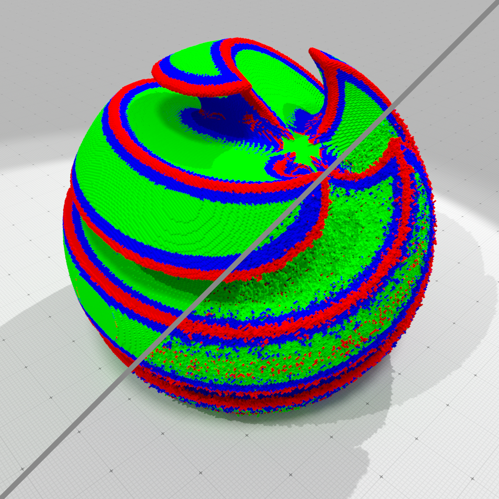
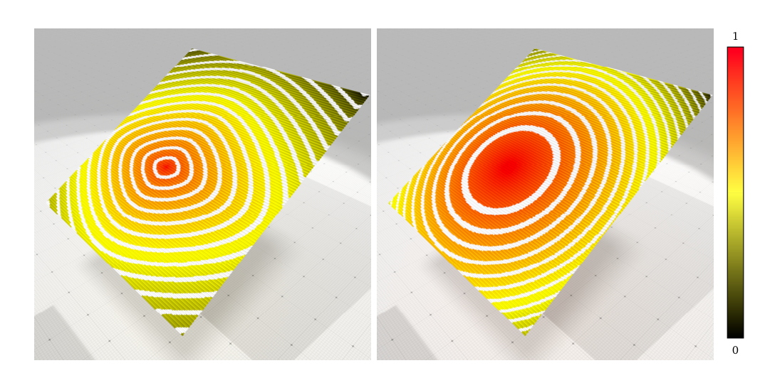
Normal vector field $u$
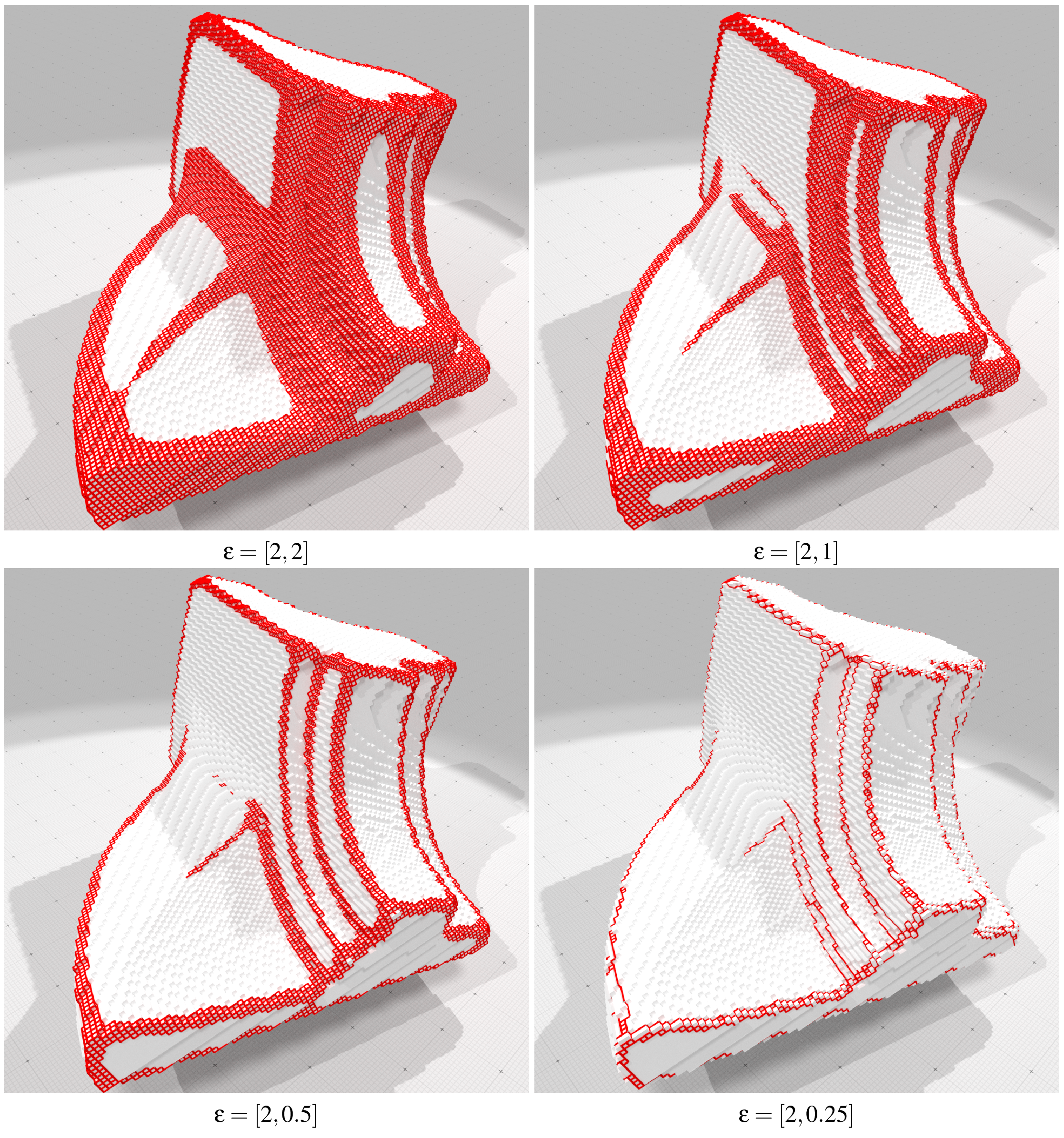
$\lambda$ parameter
$\epsilon$ parameter
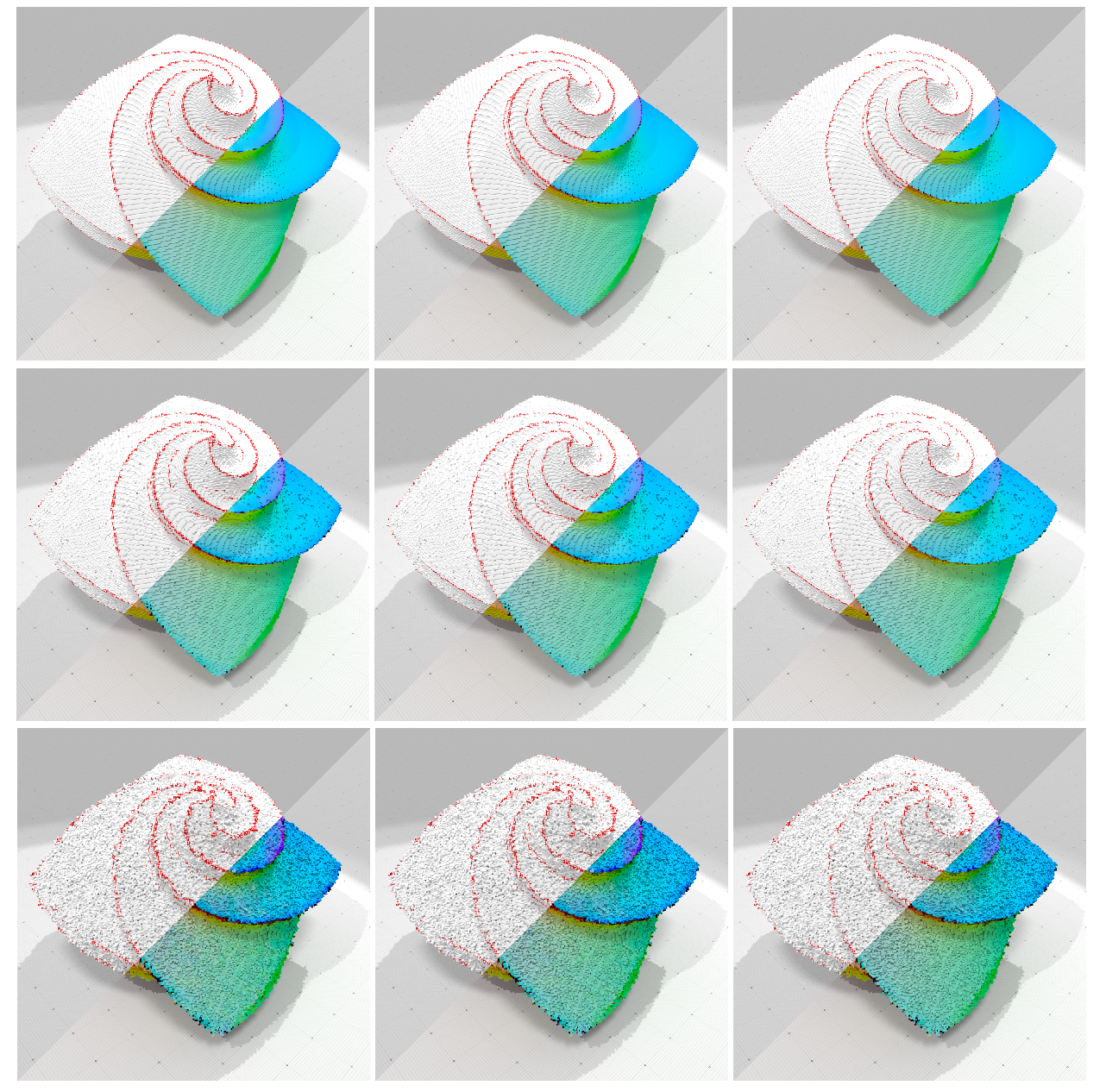
Noise level w.r.t. $\alpha$ parameter
In summary
- Anisotropic normal vector field regularization with feature selection
- Sharp features
- Parameters make sense :)
- Variational problem discretization using combinatorial representation of the digital surface
AT functional for mesh processing
Denoising, inpainting, mesh segmentation, normal map embossing...
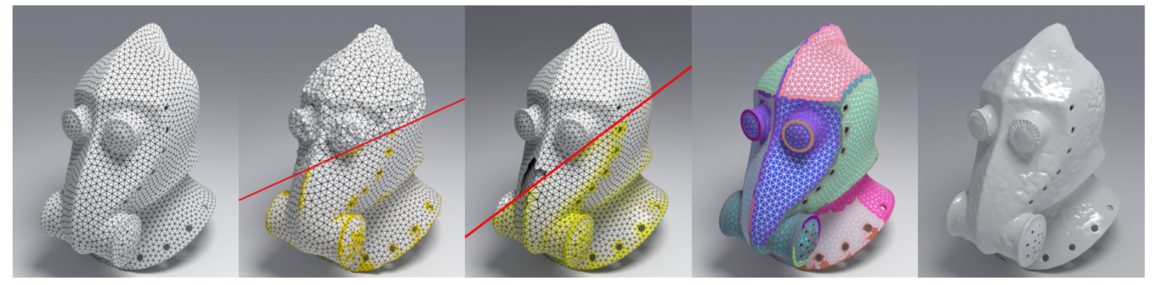 [Bonneel, C., Gueth, Lachaud]
Laplace-Beltrami operator on digital surfaces
(with T. Caissard,
J.-O. Lachaud and T. Roussillon)
Laplace-Beltrami operator for geometry processing
with Cartesian coordinates, $\Delta u = \sum_i \frac{\partial^2 u}{\partial x_i^2}$
Principles
share state-of-the-art and cutting-edge algorithms from digital geometry community.
- easy comparisons with the state-of-the-art
- allows new-comers in the field to get started
- fast prototyping of specific softwares (material sciences, medical imaging)
- provides nice illustrations/outputs of data structures and algorithms
The Project
- C++, cross-platform (linux,mac,win), generic programming
- open-source (LGPL)
- user-guides and technical documentation, tutorials
- extensibility: can be part of image processing pipeline (e.g. itk.org)
Support from:

Symposium on Geometry Processing Software Award in 2016 !
DGtal Packages
$\mathbb{Z}^d$ 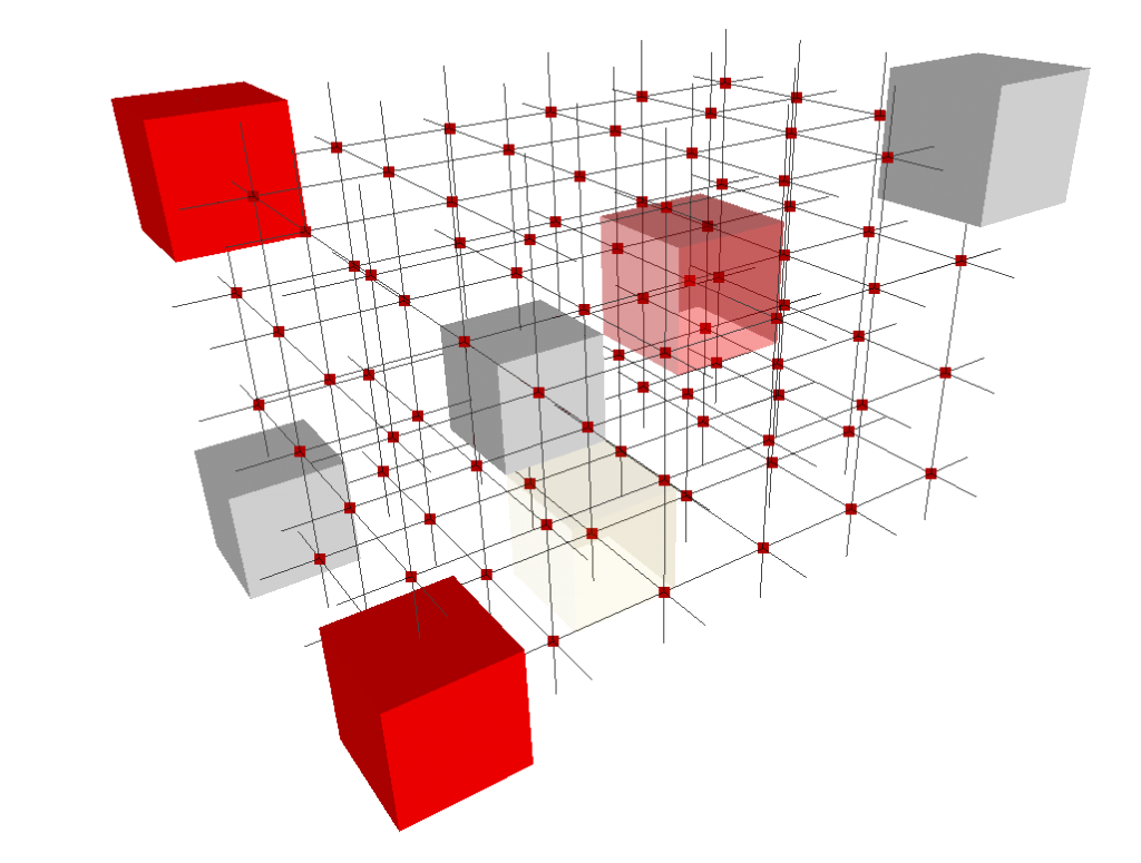 |
$u_0+\frac{1}{u_1+\frac{1}{\ldots+\frac{1}{u_k}}}$ 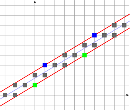 |
  |
  |
  |
| Kernel | Arithmetic | Geometry | Shapes | Topology |
|---|---|---|---|---|
 |
 |
$$Ax=b$$  |
 |
  |
| DEC | Graph | Mathematics | Image | IO |
Active community
Conclusion
Conclusion
- because input objects are given on $\Z^d$
- very efficient processing using the regularity or arithmetical properties of the data
- exact geometrical predicates
- digitization process as a specific (but relevant) discrete $\leftrightarrow$ continuous mapping
- we can do calculus
- trivial CSG operations
- efficient storage / rendering
- ...
$\Z^d$ = 😁
geometry, computer graphics, applied math, topology, arithmetic, combinatorics, image processing...
DGtal / dgtal.org