Geometry Processing on Voxel Objects
David Coeurjolly
CNRS, Université de Lyon
Digital geometry model in one slide
Topology and geometry processing of objects defined on regular lattices
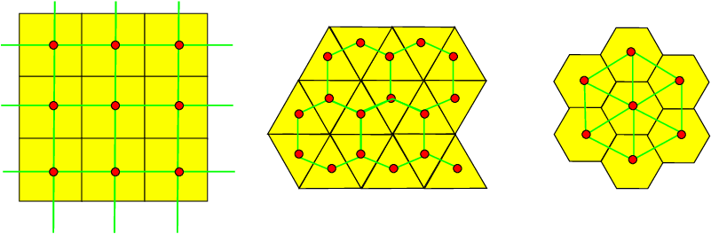
- Digital Objects = subsets of $\mathbb{Z}^d$
- Geometrical predicates = integer only computations
- $\Rightarrow$ strong impact of arithmetical properties
- Digital Topology = adjacency relationship induced by the lattice
- Digital surfaces = cells of a Cartesian cubical complex
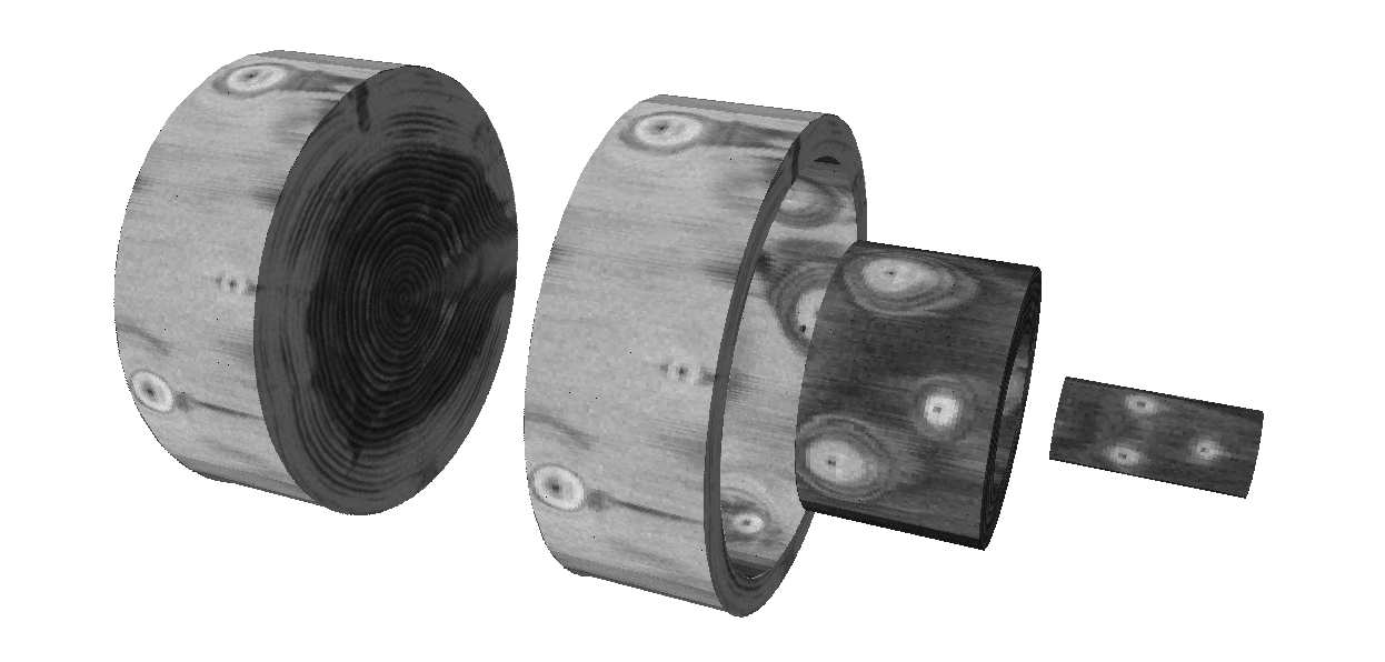
Material Sciences Applications
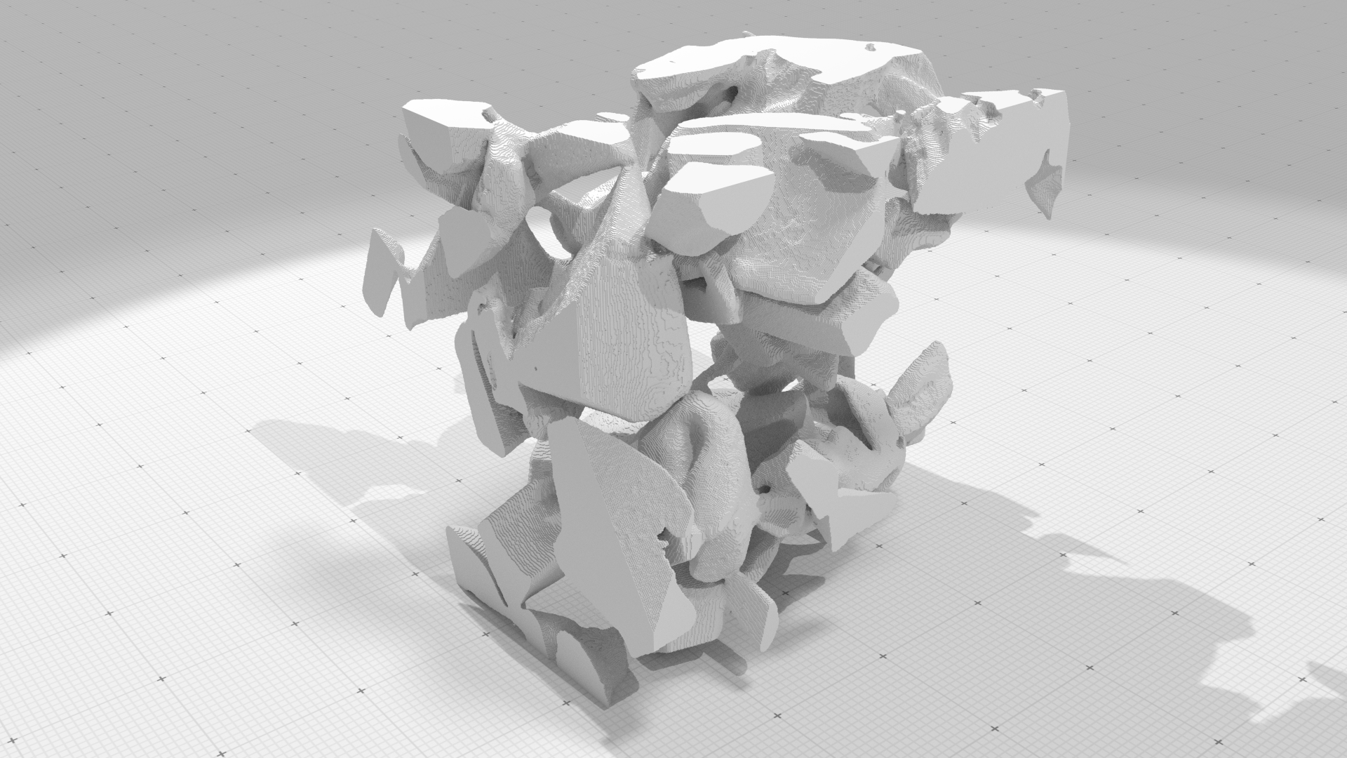

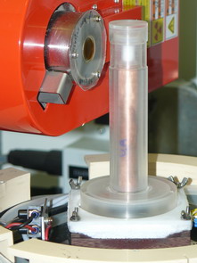
3SR Lab and CEN/CNRM - GAME URA 1357/Météo-France - CNRS
Up to $2048^3$
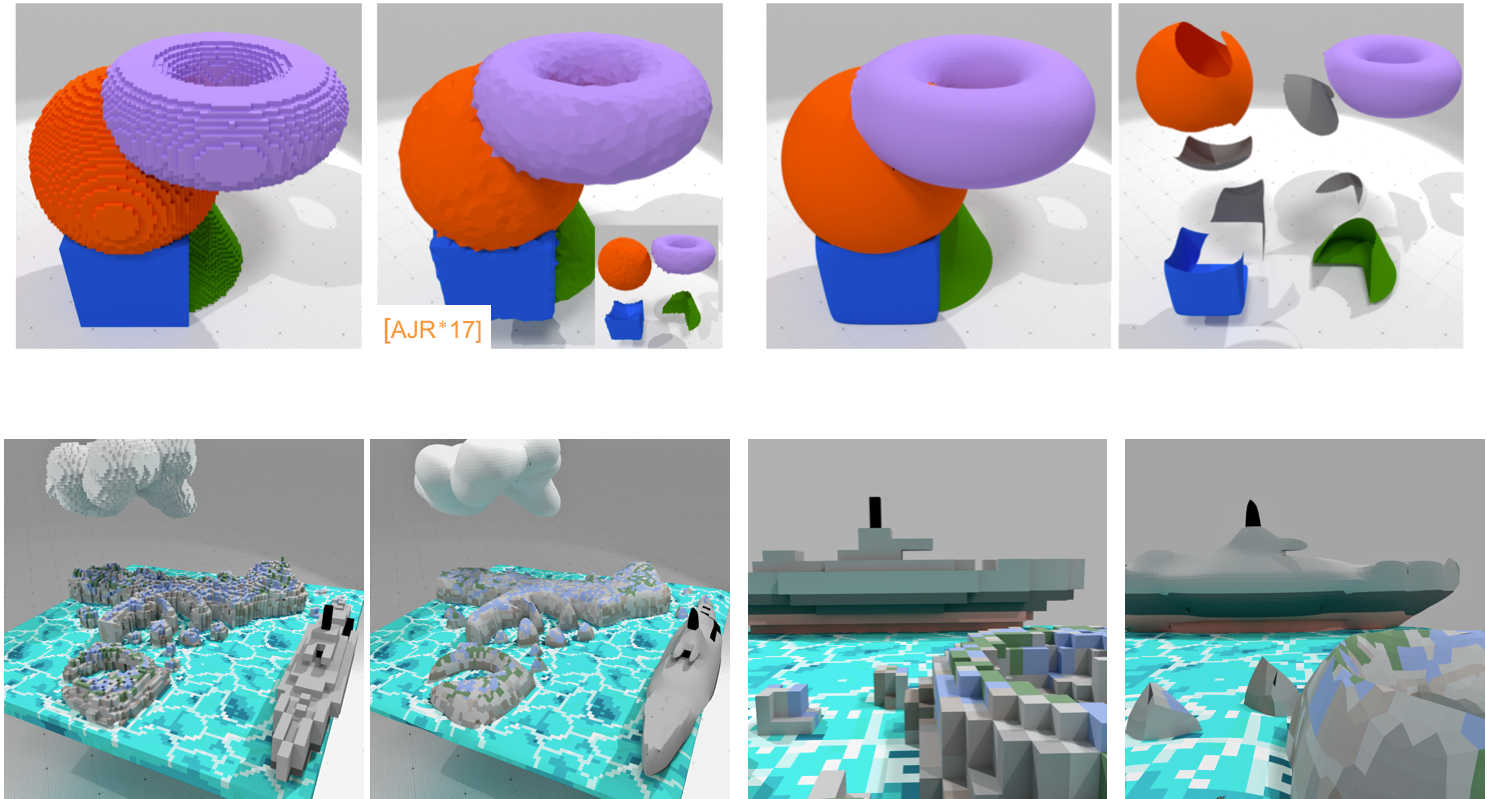
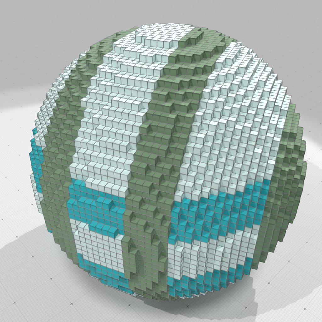
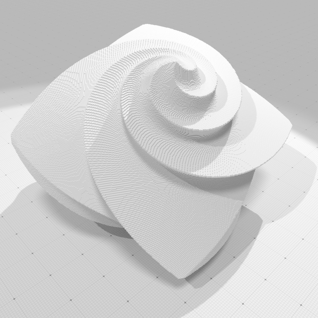
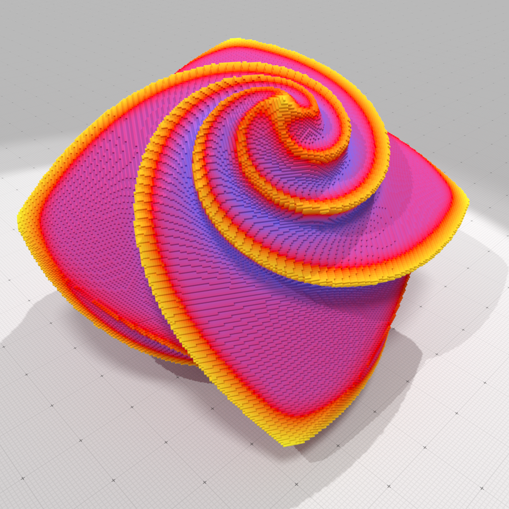
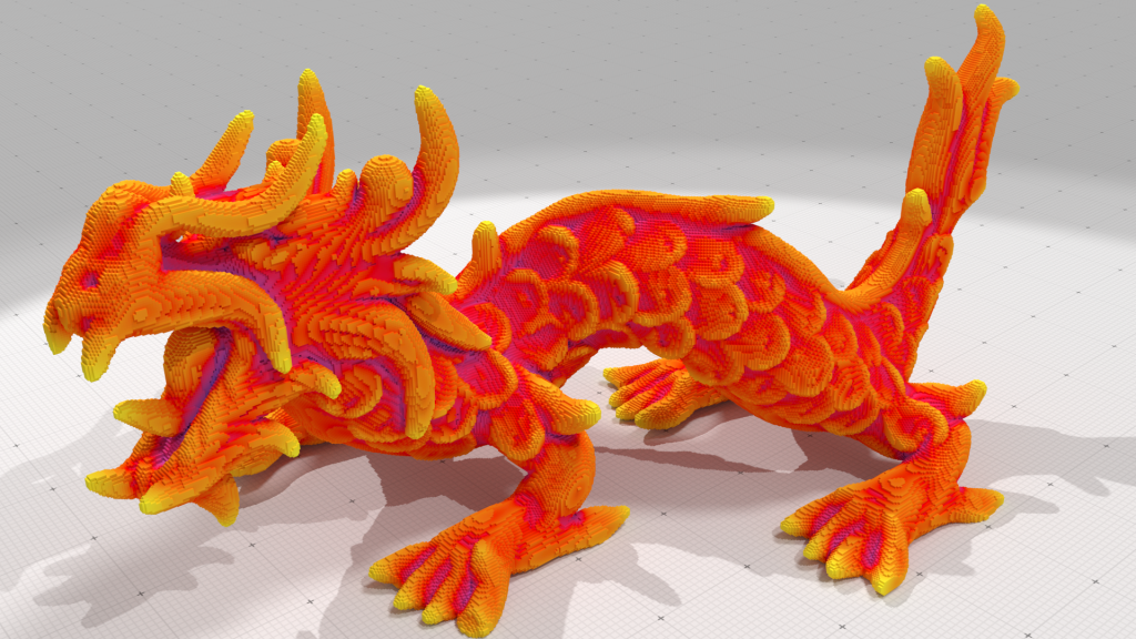
Voxel objects in computer graphics
- Widely used in geometric modeling and rendering to represent complex and interactive scenes
- Nice mathematical modeling framework
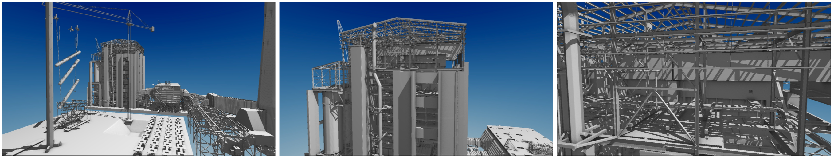
$64K^3$ voxel grid!
Villanueva, Alberto Jaspe, Fabio Marton, and Enrico Gobbetti. "SSVDAGs: symmetry-aware sparse voxel DAGs." In Proceedings of the 20th ACM SIGGRAPH Symposium on Interactive 3D Graphics and Games, pp. 7-14. ACM, 2016.
Outline
- Digital surface reconstruction
- Curvature tensor estimation
- Variational geometry processing: Ambrosio-Tortorelli functional
Collaborators: Jacques-Olivier Lachaud (Chambéry), Tristan Roussillon (Lyon), Nicolas Bonneel (Lyon), Jérémy Levallois (Lyon), Thomas Caissard (Lyon), Marion Foare (Lyon)
C., Jacques-Olivier Lachaud, Jérémy
Levallois. "Multigrid Convergent Principal Curvature Estimators in
Digital Geometry". Computer Vision and Image Understanding,
129(1):27-41, June 2014.
Thomas Caissard, C., Jacques-Olivier Lachaud, Tristan Roussillon. "Laplace–Beltrami Operator on Digital Surfaces". Journal of Mathematical Imaging and Vision, 2018.
C., Marion Foare, Pierre Gueth, Jacques-Olivier
Lachaud. "Piecewise smooth reconstruction of normal vector field on
digital data". Computer Graphics Forum (Proceedings of Pacific
Graphics), 35(7), September 2016.
Nicolas Bonneel, C., Pierre Gueth, Jacques-Olivier
Lachaud. "Mumford-Shah Mesh Processing using the Ambrosio-Tortorelli
Functional". Computer Graphics Forum (Proceedings of Pacific
Graphics), 37(7), October 2018.
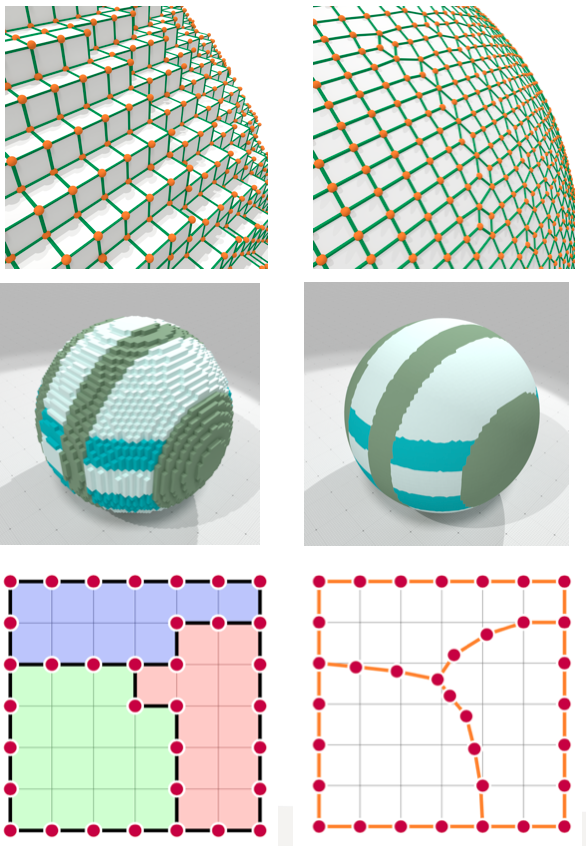
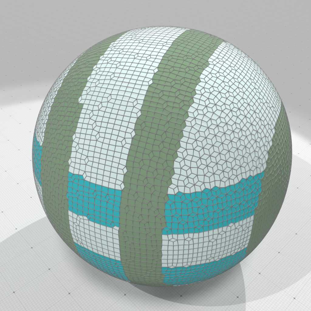
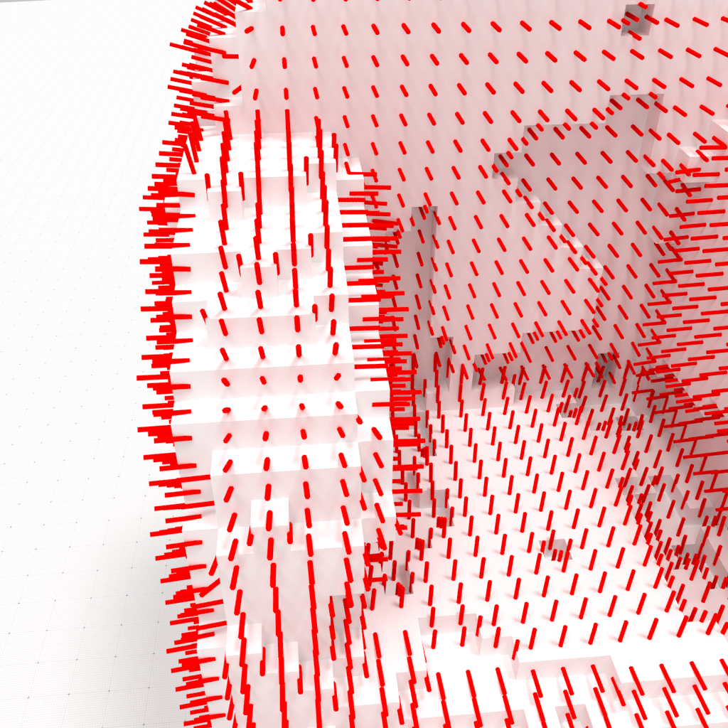
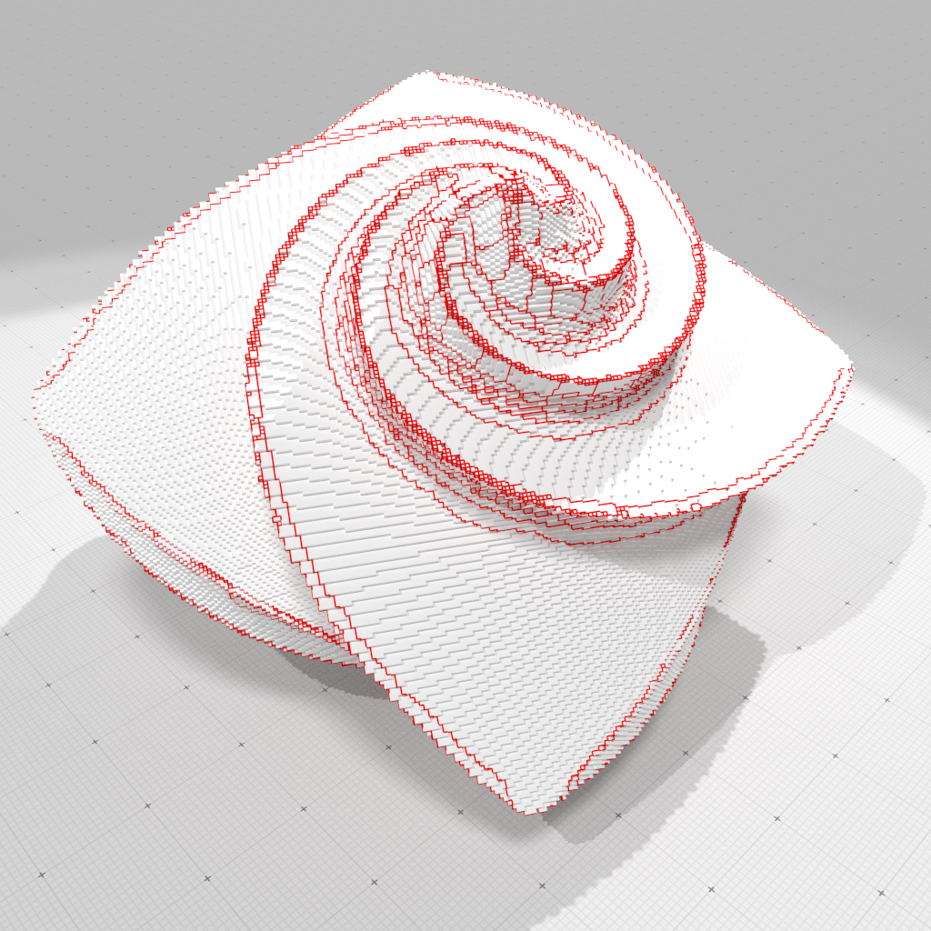
Digital Surface Regularization
Objectives
 |
|
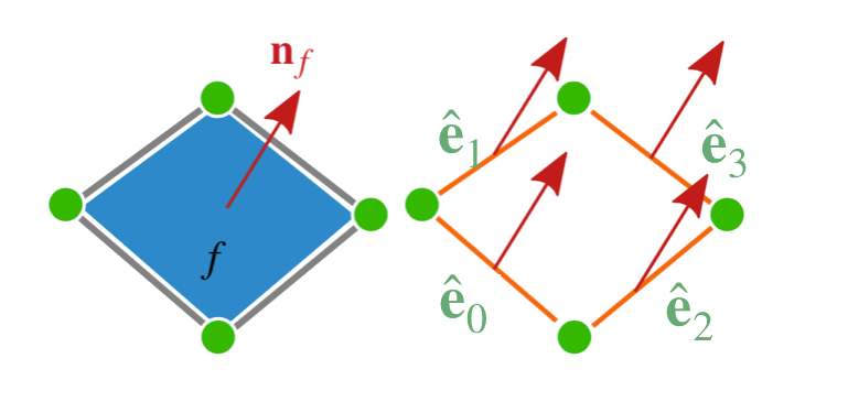
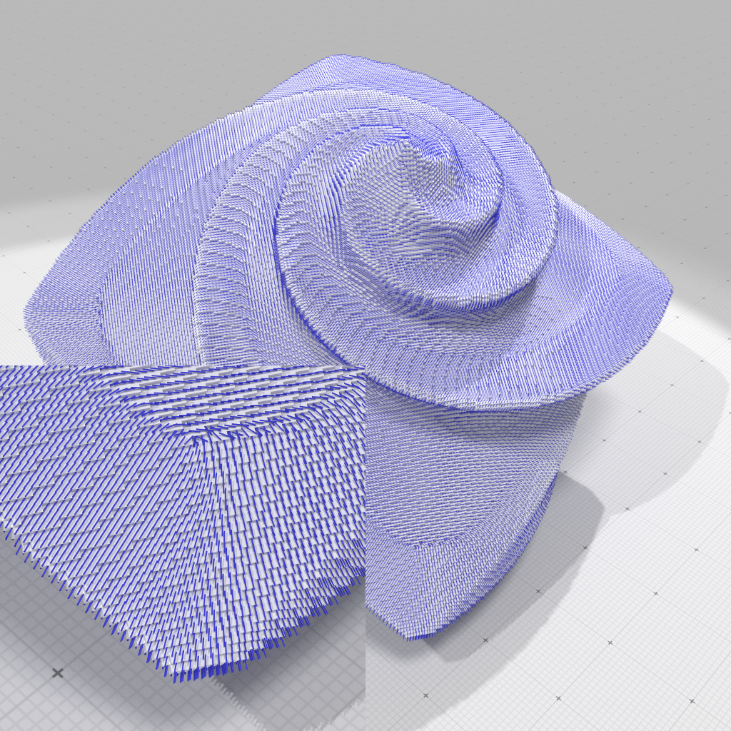
Input: consistent normal vector field $\{\mathbf{n}_{f}\}$
Variational approach
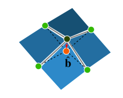
$\mathbf{p}_i$: vertices of the input digital surface, $\mathbf{n}_f$: normal vector per face
$\hat{\mathbf{p}}_i$: regularized vertices, $\hat{\mathbf{e}}_j$: edge between two regularized vertices, $\hat{\mathbf{b}}_i$: barycenter of the four adjacent regularized vertices of $\hat{\mathbf{p}}_i$ vertices
Variational approach
$\mathbf{p}_i$: vertices of the input digital surface, $\mathbf{n}_f$: normal vector per face
$\hat{\mathbf{p}}_i$: regularized vertices, $\hat{\mathbf{e}}_j$: edge between two regularized vertices, $\hat{\mathbf{b}}_i$: barycenter of the four adjacent regularized vertices of $\hat{\mathbf{p}}_i$ vertices
Data attachment
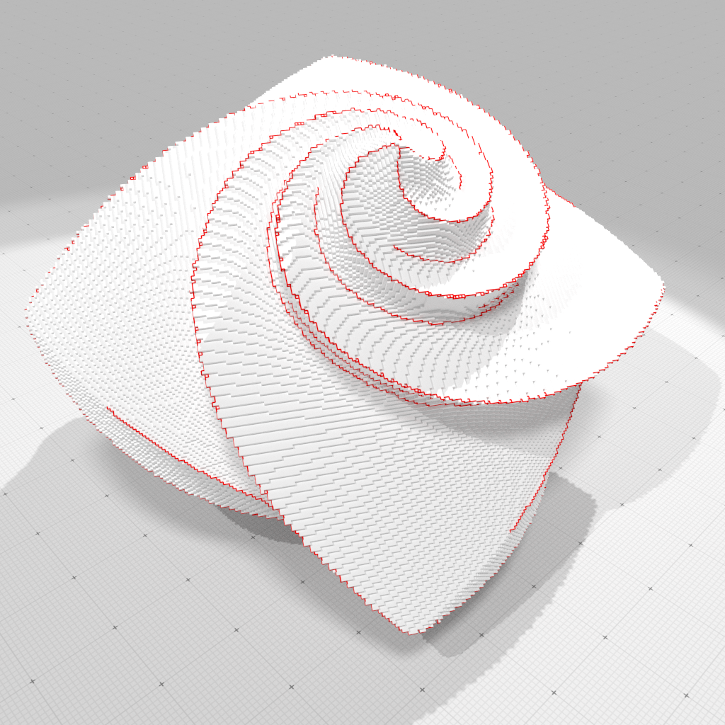
Variational approach
$\mathbf{p}_i$: vertices of the input digital surface, $\mathbf{n}_f$: normal vector per face
$\hat{\mathbf{p}}_i$: regularized vertices, $\hat{\mathbf{e}}_j$: edge between two regularized vertices, $\hat{\mathbf{b}}_i$: barycenter of the four adjacent regularized vertices of $\hat{\mathbf{p}}_i$ vertices
Data attachment + Quad alignement
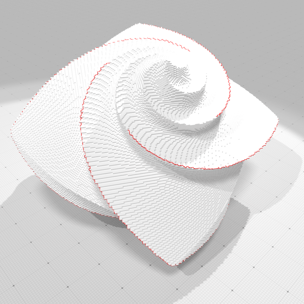
Variational approach
$\mathbf{p}_i$: vertices of the input digital surface, $\mathbf{n}_f$: normal vector per face
$\hat{\mathbf{p}}_i$: regularized vertices, $\hat{\mathbf{e}}_j$: edge between two regularized vertices, $\hat{\mathbf{b}}_i$: barycenter of the four adjacent regularized vertices of $\hat{\mathbf{p}}_i$ vertices
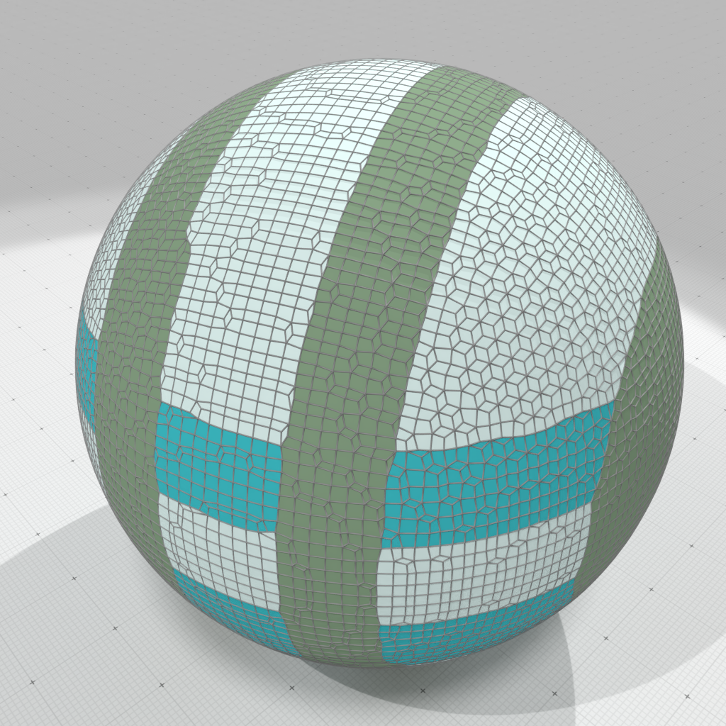
Data attachment + Quad alignement + Fairness term
Minimizing the energy
$\Rightarrow$ Optimal position given by solving a linear system
$\Rightarrow$ Efficient interactive regularization on GPU 😀
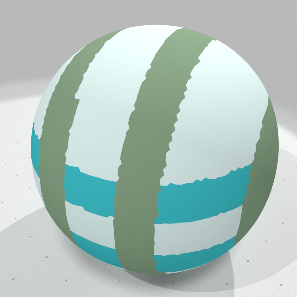
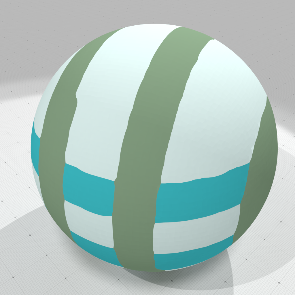
Multilabel case

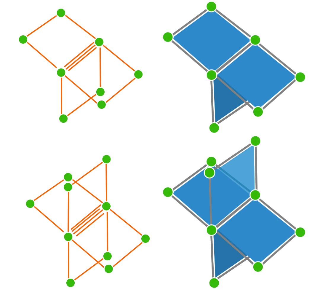
$\Rightarrow$ Same formulation and trivial regularization thanks to the grid structure
Tweaking the fairness term
 |
 |
 |
 |
 |
 |
Digital Geometry point of view: theoretical guarantees
If $M$ is smooth (positive reach) and $M_h:=M\cap ( h\cdot\mathbb{Z}^3)$ its digitization on a grid with gridstep $h$, then $$ \frac{1}{n}\sum_{i=1}^{n} \|\mathbf{p}^*_i - \mathbf{p}_i\| \leq C\cdot h \quad\quad \frac{1}{n}\sum_{i=1}^{n}\,d(\mathbf{p}^*_i, \partial M) \leq C'\cdot h$$
If normal vectors $\{\mathbf{n}_ƒ\}$ are multigrid convergent, normal vectors to regularized quads are also multigrid convergent and we have an even better approximation of $\partial M$
wait..."gridstep?" "Multigrid convergent vector field?"
Curvature Tensor Estimation
Digitization model
Given $\Shape \subset \R^d$, its digitization at gridstep $h$ is $$\DigF{\Shape}{h} = \left(\frac{1}{h} \cdot \Shape\right) \cap \Z^d$$
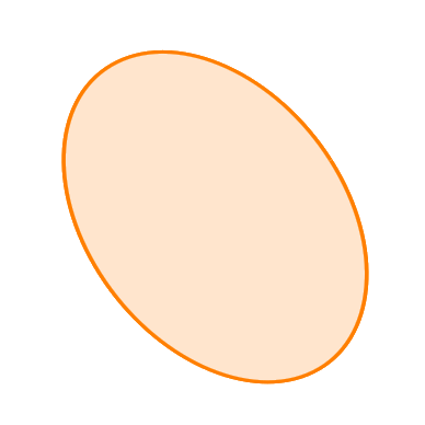
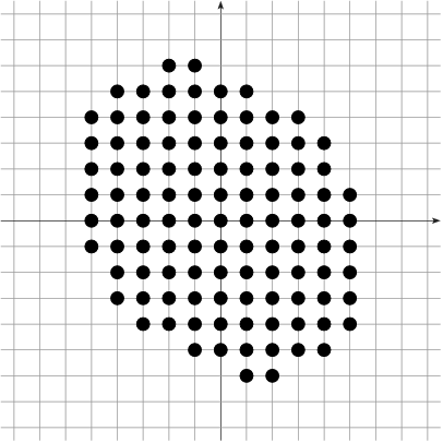
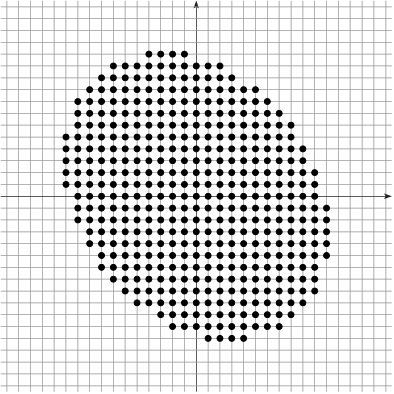
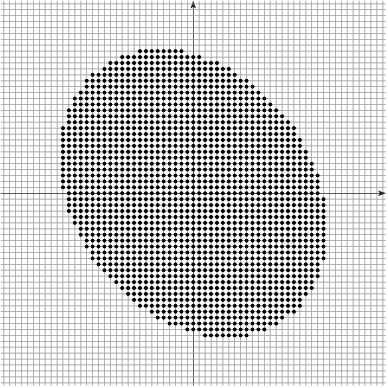
Example: $h^2|\DigF{\Shape}{h}|$ converges to the measure of $\Shape$ as $h\rightarrow 0$
[Gauss, Dirichlet, Huxley...]
Multigrid convergence of a local estimator
Given a digitization process $\AnyDig$, a local discrete geometric
estimator $\hat{E}$ of some geometric quantity $E$ is multigrid
convergent for the family of shapes $\Shapes$ if and only if, for any $\Shape
\in \Shapes$, there exists a grid step $h_\Shape>0$ such that the
estimate $\hat{E}(\AnyDig_{\Shape}(h),\hat{\vx},h)$ is defined for all
$\hat{\vx} \in \Bd{\Body{\AnyDig_{\Shape}(h)}{h}}$ with $0< h< h_\Shape$, and for
any $\vx \in \dS$,
$$
\forall \hat{\vx} \in \Bd{\Body{\AnyDig_{\Shape}(h)}{h}} \text{ with } \| \hat{\vx} -\vx\|_\infty
\le h, \quad\quad \color{myred}{|
\hat{E}(\AnyDig_{\Shape}(h),\hat{\vx},h) - E(\Shape,\vx) | \le \tau_{\Shape,\vx}(h)},
$$
where $\tau_{\Shape,\vx}: \R^{+} \setminus\{0\} \rightarrow \R^+$ has null limit at
$0$. The convergence is uniform for
$\Shape$ when every $\tau_{\Shape,\vx}$ is bounded from above by a function
$\tau_\Shape$ independent of $\vx \in \Bd{\Shape}$ with null limit at $0$.
Digital/Continuous mapping

-
The Hausdorff between $\partial \Shape$ and $\partial_h\Shape$ is
bounded by $\sqrt{d}h/2$
- For $d=2$, there exists an homeomorphism between $\partial X$ and $\partial_h X$
- For $d\geq 3$, no homeomorphism ☹, but
- Projection operator $\xi:\,\partial_h\Shape\rightarrow\partial \Shape$ is surjective
- Area of non-injective parts of $\xi$ the tends to zero
Digitization as an Hausdorff sampling of the continuous object

Can we estimate the curvature tensor on digital surfaces with multigrid convergence properties ?
Huge literature on differential quantity estimators
- Meshes
- Local estimators (1- ou 2-rings) [Surazhsky et al. 2003][Gatzke, Grimm 2006]
- Gauss-Bonnet formula based estimators [Xu 2006]
- Normal cycles [Cohen-Steiner, Morvan 2006]
- Point Clouds
- Jet-Fitting approaches [Cazals, Pouget 2005]
- Voronoi cell covariance measure (VCM) [Alliez et al. 2007][Merigot et al. 2011][Cuel et al. 2014]
- Generic framework
- Varifold approaches [Buet 2014][Buet et al. 2015]
→ accuracy depends on the mesh/point cloud quality
→ incompatible constraints on convergence theorem w.r.t. digital surface
Main contributions: Integral Invariant approach
If $\Shape$ is compact and $\partial \Shape$ has positive reach $\rho$ and $C^3$-continuity then
- Mean curvature and principal curvature estimations converge in $O(h^{\frac{1}{3}})$
- Normal vector field estimation converges in $O(h^{\frac{2}{3}})$
- Principal Curvature directions converge in $\frac{1}{|\PrincCurv{1}(\Shape,\vx)-\PrincCurv{2}(\Shape,\vx)|} O(h^{\frac{1}{3}})$


Overall proof scheme
${\kappa}(\Shape,\vx) \EqDef \underbrace{\frac{3\pi}{2{{R}}} - \frac{3\cdot { A_R(\Shape,\vx)}}{{{R}}^3}}_{ \tilde{\kappa}^{R}(\Shape,\vx) } + O(R)$ [Pottmann et al. 2007]
→ $A_R(\Shape,\vx) \rightarrow \AreaC(\Ball{R/h}{\vx/h} \cap \DigF{\Shape}{h})$
+ [Pottmann et al. 2007] $\quad\CurvH{R}(\DSh,\vx,h)$
→ $\CurvH{R}(\DSh,\hat{\vx},h) \rightarrow \Curv(\Shape,\vx)$
Area estimator "à la" Gauss
\[ {\color{myblue}\AreaC(\DSh)} \EqDef h^2 \Card (\DSh) \]
$\quad \AreaC(Y) = \Area(\Shape) + {\color{myblue}O(h^\beta)}\quad\quad\text{with}\quad \beta \ge 1$
- $\beta = 1$ for $\Shapes^C$ [Gauss, Dirichlet]
- $\beta = \frac{15}{11}-\epsilon$ for $\Shapes^{3-SC}$ (non null curvature) [Huxley 1990]
Area estimator "à la" Gauss
\[ {\color{myblue}\AreaC(Y)} \EqDef h^2 \Card (Y) \quad\quad\text{with}\quad Y = \Ball{R/h}{\vx/h} \cap \DigF{\Shape}{h} \]
$\quad \AreaC(Y) = A_R(\Shape,\vx) + {\color{myblue}O(h^\beta R^{2-\beta})} \quad\quad\text{with}\quad \beta \ge 1$


Overall proof scheme - 1/3
→ $A_R(\Shape,\vx) \rightarrow \AreaC(\Ball{R/h}{\vx/h} \cap \DigF{\Shape}{h})$

+ [Pottmann et al. 2007] $\quad\CurvH{R}(\DSh,\vx,h)$
→ $\CurvH{R}(\DSh,\hat{\vx},h) \rightarrow \Curv(\Shape,\vx)$
Curvature estimation by digital integration
\[ \hat{\kappa}^{R}(\DigF{\Shape}{h},\vx,h) \EqDef \frac{3\pi}{2{{R}}} - \frac{3 {\color{myblue}\AreaC(Y)}}{{{R}}^3} {\color{mydarkred}+O(R)} \quad\text{with}\quad Y = \Ball{R/h}{\vx/h} \cap \DigF{\Shape}{h} \]
Overall proof scheme - 2/3
→ $A_R(\Shape,\vx) \rightarrow \AreaC(\Ball{R/h}{\vx/h} \cap \DigF{\Shape}{h})$
+ [Pottmann et al. 2007] $\quad\CurvH{R}(\DSh,\vx,h)$
→ $\CurvH{R}(\DSh,\hat{\vx},h) \rightarrow \Curv(\Shape,\vx)$
Positioning Error

― $\pi^\Shape_h(\hat{\vx})$

Multigrid convergence of the digital curvature estimator
→ Setting $R=kh^\alpha$, we select $\alpha$ to minimize all errors.
Curvature tensor on digital surfaces

\[ \begin{align} &\PrincCurvH{1}{R}(\DSh,\vx,h) \EqDef \frac{6}{\pi R^6}\left({\color{myblue}\hat{\lambda}_2} - 3{\color{myblue}\hat{\lambda}_1}\right) + \frac{8}{5R}\\ &\PrincCurvH{2}{R}(\DSh,\vx,h) \EqDef \frac{6}{\pi R^6}\left({\color{myblue}\hat{\lambda}_1} - 3{\color{myblue}\hat{\lambda}_2}\right) + \frac{8}{5R}\\ &\PrincDirH{1}{R}(\DSh,\vx,h) \EqDef {\color{myblue}\hat{\nu}_1}\\ &\PrincDirH{2}{R}(\DSh,\vx,h) \EqDef {\color{myblue}\hat{\nu}_2}\\ &\NormalDirH{R}(\DSh,\vx,h) \EqDef {\color{myblue}\hat{\nu}_3} \end{align} \]
$\{{\color{myblue}\hat\nu_i,\hat\lambda_i}\}$ are the eigenvalues/eigenvectors of the covariance matrix of $B_r(\vx)\cap \Shape$
\[ \begin{align} &\exists h_\Shape \in \R^+,\,\, \forall h \in \R,\,\, 0 < h < h_\Shape,\,\, \,\,\nonumber\quad \quad\quad \quad\\ &\forall \vx \in \Bd{\Shape}, \quad \forall \hat{\vx} \in \Bd{\Body{\DSh}{h}} \text{ avec } \| \hat{\vx} -\vx\|_\infty \le h, \nonumber\quad \quad\quad \quad \\ &\quad \quad\quad \quad\| \PrincDirH{1}{R}( \DSh, \hat{\vx}, h ) - \PrincDir{1}(\Shape, \vx) \| \le \frac{1}{|\PrincCurv{1}(\Shape,\vx)-\PrincCurv{2}(\Shape,\vx)|} O(h^{\frac{1}{3}})\,, \\ &\quad \quad\quad \quad\| \PrincDirH{2}{R}( \DSh, \hat{\vx}, h ) - \PrincDir{2}(\Shape, \vx) \| \le \frac{1}{|\PrincCurv{1}(\Shape,\vx)-\PrincCurv{2}(\Shape,\vx)|} O(h^{\frac{1}{3}})\,, \\ &\quad \quad\quad \quad\| \NormalDirH{R}( \DSh, \hat{\vx}, h ) - \NormalDir(\Shape, \vx) \| \le O(h^{\frac{2}{3}})\,. \end{align} \]
In summary
- Robust, efficient implementation (convolutions)
- Parametrized by a integration radius $R$ or a grid step $h$
- Proof relies on digital/continuous relationships and geometrical moment estimation
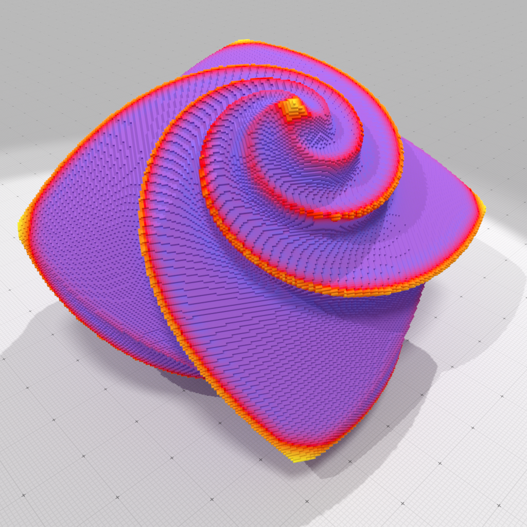
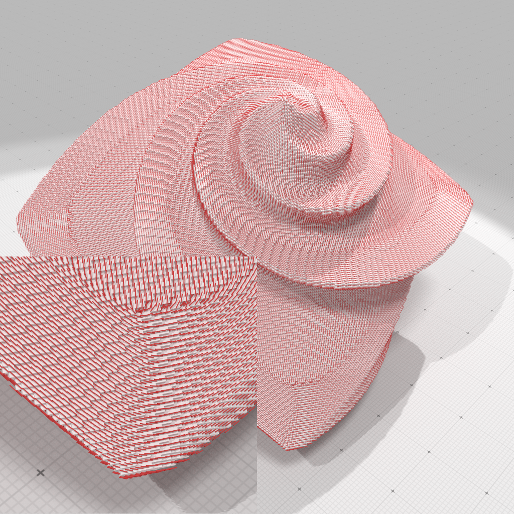
Piecewise smooth reconstruction
Problem statement
 $\Rightarrow$ Piecewise smooth reconstruction of the normal
vector field
$\Rightarrow$ Piecewise smooth reconstruction of the normal
vector field
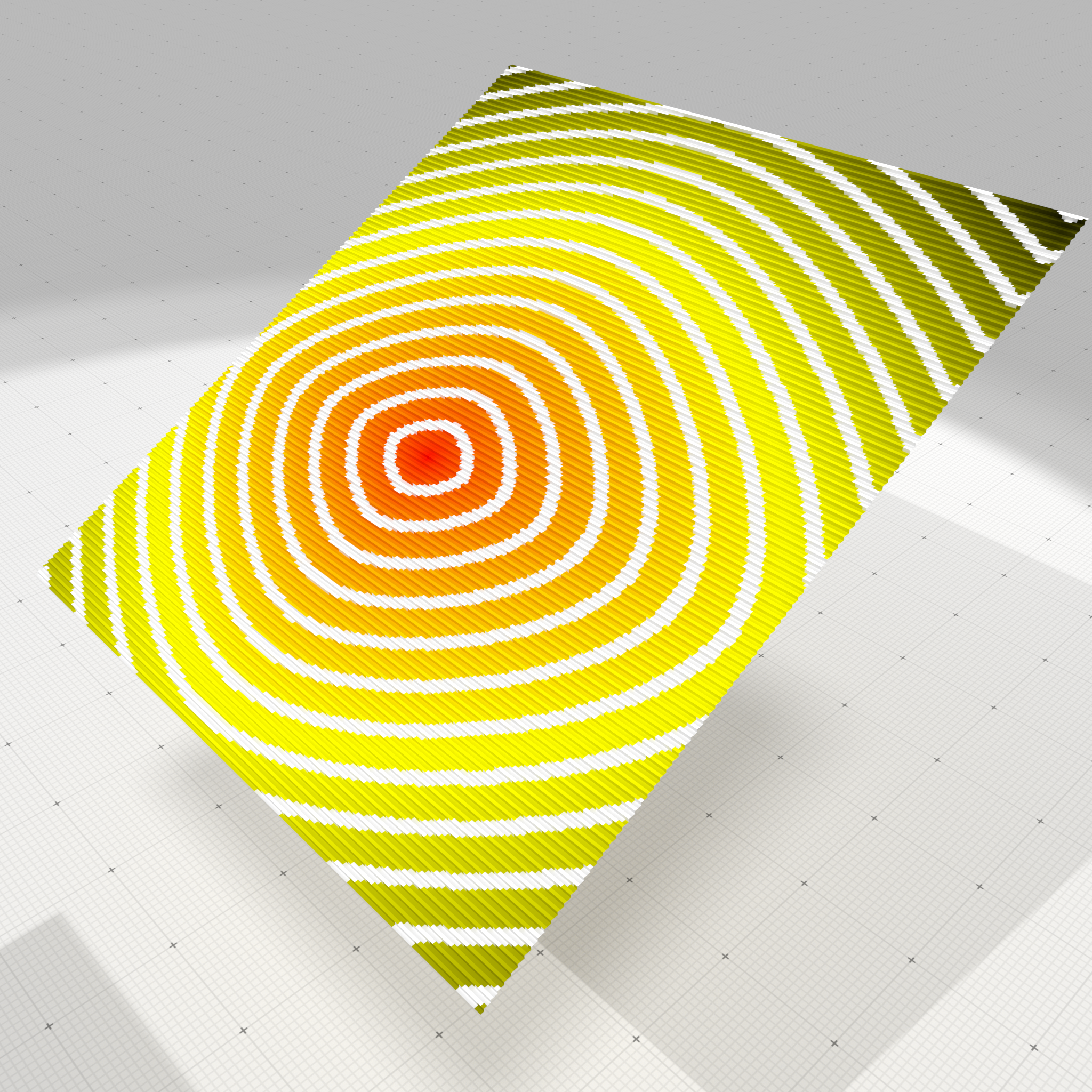
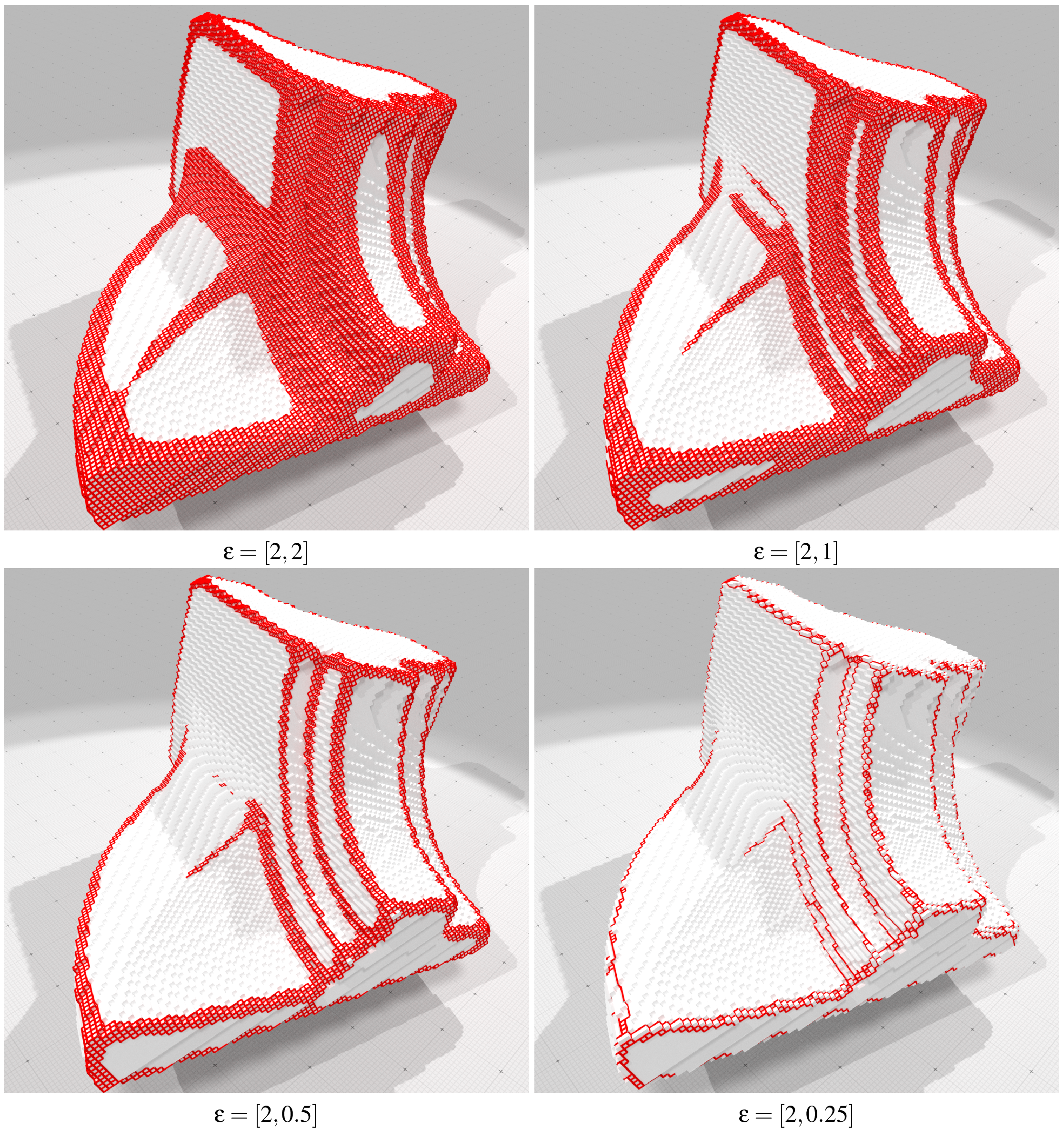
Ambrosio-Tortorelli functional
$$ \mathcal{AT}_\eps(u,v) = {\alpha} \underbrace{\dint_{{M}} |u - g|^{{2}} \dx}_{\text{attachment term}} + \underbrace{\dint_{{M}} |{v} \grad u|^{{2}} \dx}_{\text{smoothness term}} + \underbrace{{\lambda} \dint_{{M}} {\eps} |\grad {v}|^{{2}} + \frac{1}{4 {\eps}} |1 - {v}|^{{2}} \dx}_{\text{discontinuity length}}$$
- Two functions to optimize: $u$ (scalar map) and $v$ (feature scalar map, $\mathcal{M}\rightarrow [0,1]$)
- $v\approx 1$ on smooth parts, $v\approx 0$ near features
- Quadratic terms
- the AT functional $\Gamma-$converges to Mumford-Shah's functional $\mathcal{AT}_\eps \gammaconv{\eps \to 0} \mathcal{MS}$
- (integration domain does not change, no Hausdorff measure)
Ambrosio-Tortorelli functional
$$ \mathcal{AT}_\eps(u,v) = {\alpha} \underbrace{\dint_{{M}} |u - g|^{{2}} \dx}_{\text{attachment term}} + \underbrace{\dint_{{M}} |{v} \grad u|^{{2}} \dx}_{\text{smoothness term}} + \underbrace{{\lambda} \dint_{{M}} {\eps} |\grad {v}|^{{2}} + \frac{1}{4 {\eps}} |1 - {v}|^{{2}} \dx}_{\text{discontinuity length}}$$
- $\eps$ -- thickness of the feature set ($[distance]$)
- ${\alpha}$ -- attachment coefficient to control the smoothing strength ($[area^{-1}]$)
- $\lambda$ -- proportional to the length of discontinuities ($[distance^{-1}]$)
Discretization
"à la" Discrete Exterior Calculus [Hirani, Desbrun, Grady...]:
$\mathcal{M}$ is a cellular complex ($\mathcal{M}'$ its dual), $\sigma^k$ are $k-$cells of $\mathcal{M}$ (resp. $\sigma'^k$ of $\mathcal{M}'$)


- $k-$forms are vectors of $|\{\sigma^k\}|$ scalars
- Linear operators are matrices
- e.g.
- $d_k$ (exterior derivative) maps primal $k-$forms to primal $(k+1)-$forms
- wedge product $\alpha\wedge \beta$ maps $k-$forms and $l-$forms to $(k+l)-$forms
- Hodge-star $\star_k$ operator to maps primal $k-$forms to dual $k-$forms
- ...
Discretization (bis)
$$ \mathcal{AT}_\eps(u,v) = {\alpha} \underbrace{\dint_{{M}} |u - g|^{{2}} \dx}_{\text{attachment term}} + \underbrace{\dint_{{M}} |{v} \grad u|^{{2}} \dx}_{\text{smoothness term}} + \underbrace{{\lambda} \dint_{{M}} {\eps} |\grad {v}|^{{2}} + \frac{1}{4 {\eps}} |1 - {v}|^{{2}} \dx}_{\text{discontinuity length}}$$
$v$ is a primal $0$-form, $u$ is a triple of dual $0$-forms $(u_1,u_2,u_3)$ and we discretize $\mathcal{AT}_\epsilon$
Discretization (ter)
$$\mathcal{AT}^d_\epsilon(u,v) \EqDef \alpha \sum_{i=1}^{3} \langle{u_i - g_i},{u_i - g_i}\rangle_\bar{0} + \sum_{i=1}^{3} \langle{v \wedge d_\bar{0} u_i},{v \wedge d_\bar{0} u_i}_\bar{1}\rangle_\bar{1} \\ \quad\quad\quad\quad\quad\quad\quad\quad\quad+ \lambda \epsilon \langle{ d_{0} v },{ d_{0} v }\rangle_1 + \frac{\lambda}{4\epsilon} \langle{1 - v},{1 - v}\rangle_0$$
- if $\gamma$ is a primal $0-$form and $\beta$ a dual $1-$form, then $\gamma\wedge\beta=diag(\beta)M\gamma$ with $M\EqDef\frac{1}{2}|d_0|$
- $A$ is the matrix form of $d_0$
- $B$ is the matrix form of $d_\bar{0}$
- $\vu_i,\,\vv,\,\vg$ are column vectors containing associated $k-$form scalars
- $S_i$ is a diagonal matrix encoding the Hodge star $\star_i$
$$\mathcal{AT}^d_\epsilon(\vu,\vv)= \alpha (u-g)^T S_{\bar{0}} (u-g) + u^T B^T \operatorname{Diag}(M v) S_{\bar{1}} \operatorname{Diag}(M v) B u \\ + \lambda\,\epsilon\, v^T A^T S_1 A v + \frac{\lambda}{4\epsilon} (1-v)^T S_0 (1-v)$$
Optimization
$\min_{u,v} \mathcal{AT}_\eps \Leftrightarrow \left( \nabla_u \mathcal{AT}_\eps = 0 \right) \wedge \left(\nabla_v \mathcal{AT}_\eps = 0 \right)$
For a given $\epsilon$:
$$ \nabla_u AT_\epsilon[u, v] = 0 \Leftrightarrow \left[
\alpha\,S_{\bar{0}} - B^T \operatorname{Diag}(M v) S_{\bar{1}}
\operatorname{Diag}(M v) B \right] u = \alpha\,S_{0}\,g
$$
$$\nabla_v AT_\epsilon[u, v] = 0 \Leftrightarrow
\left[ \frac{\lambda}{4\epsilon} S_0 + \lambda\,\epsilon\,A^T S_1 A + M^T \operatorname{Diag}(B u) S_{\bar{1}} \operatorname{Diag}(B u) M \right] v = \frac{\lambda}{4\,\epsilon} S_0$$
$\Rightarrow$ only linear system solves on sparse matrices !
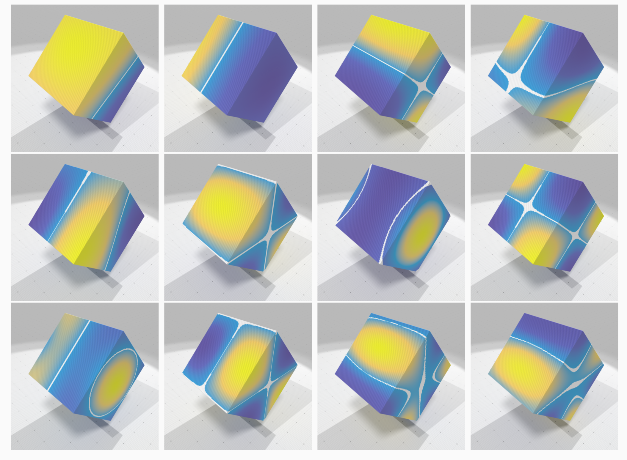
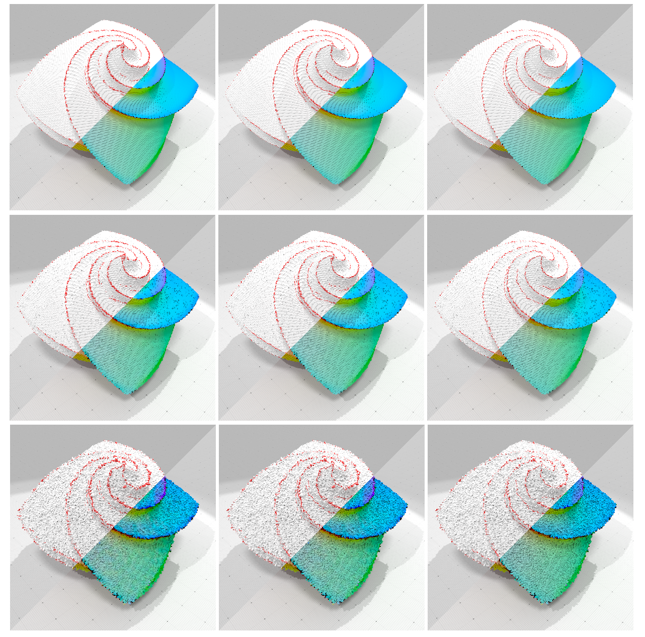
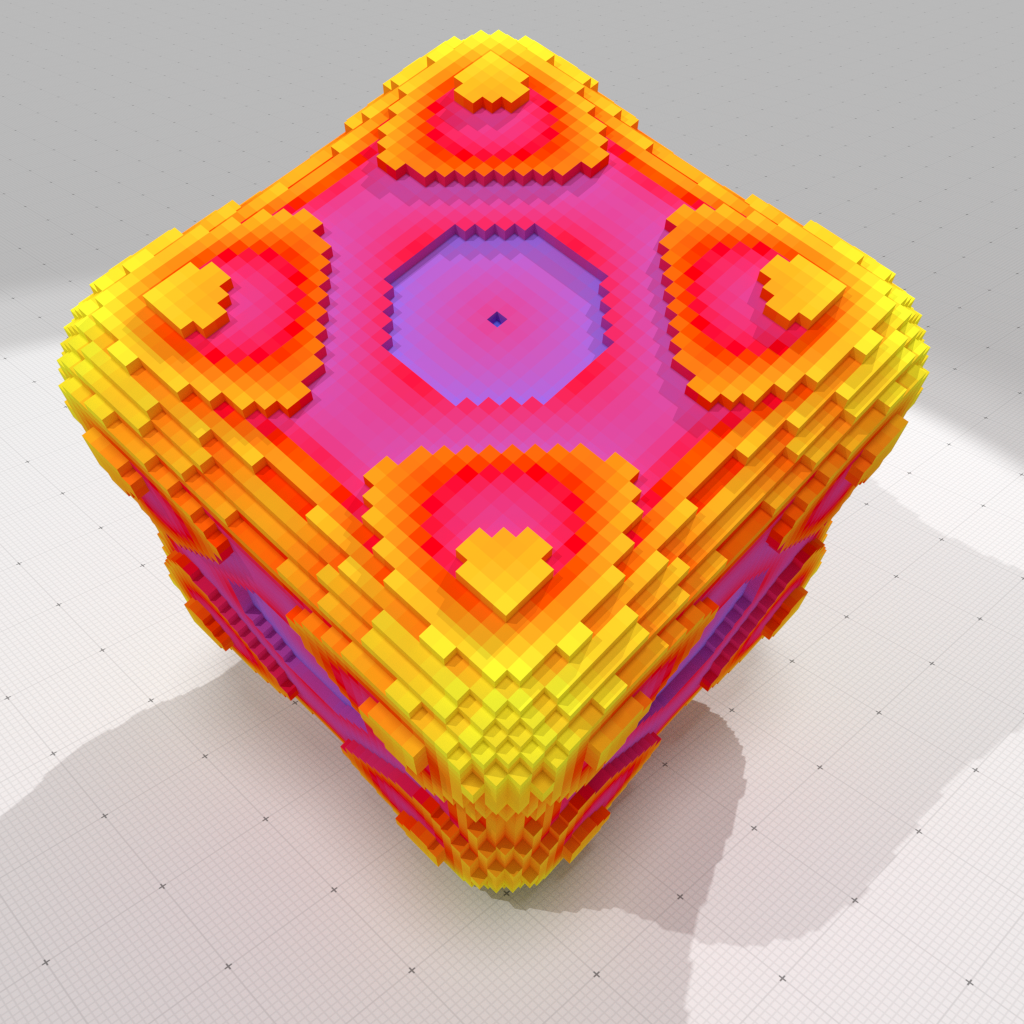
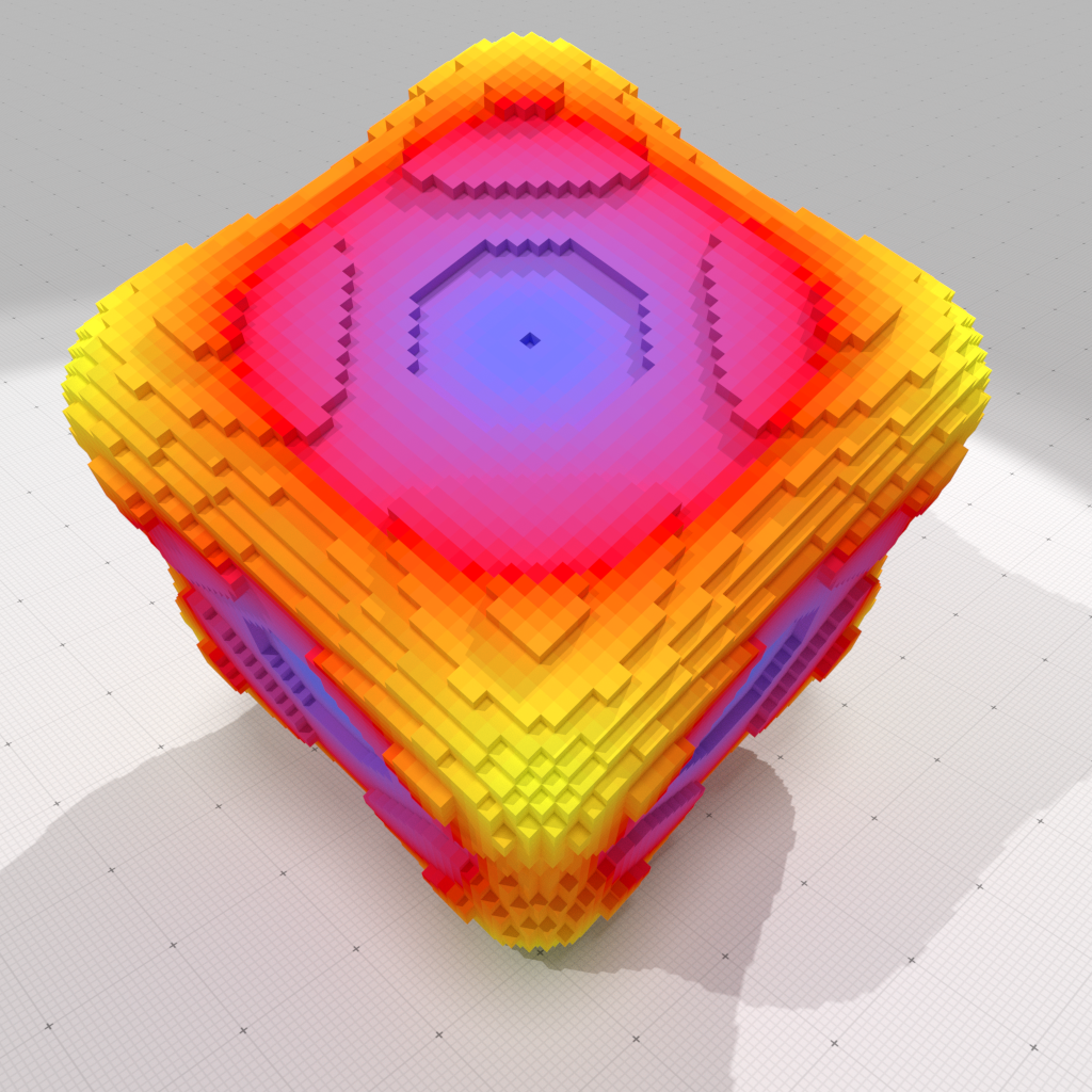
$\lambda$ parameter
$\epsilon$ parameter
Noise level w.r.t. $\alpha$ parameter
In summary
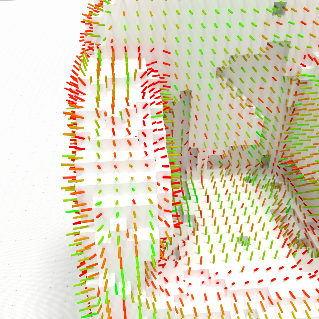
- Anisotropic normal vector field regularization with feature selection
- Sharp features
- Parameters make sense :)
- Variational problem discretization using a combinatorial representation of the digital surface
Chicken/egg problem: measure of quads $\mu(s)$ used in the DEC operators
Ambrosio-Tortorelli on meshes
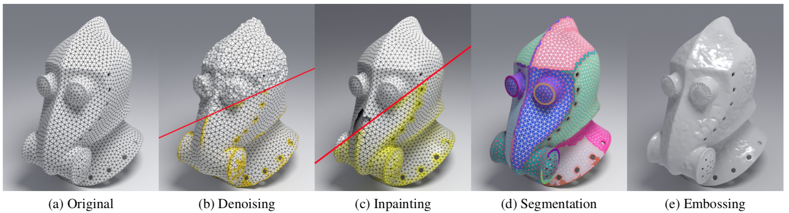
Nicolas Bonneel, C., Pierre Gueth, Jacques-Olivier Lachaud. Mumford-Shah Mesh Processing using the Ambrosio-Tortorelli Functional. Computer Graphics Forum (Proceedings of Pacific Graphics), 37(7), October 2018.
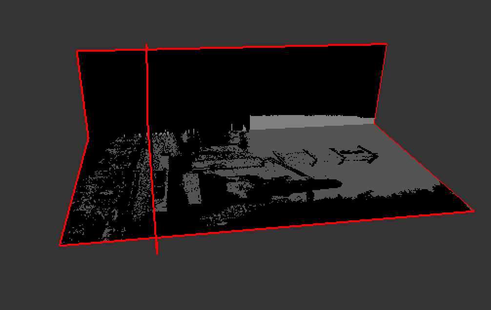
Geometrical deep learning data fusion
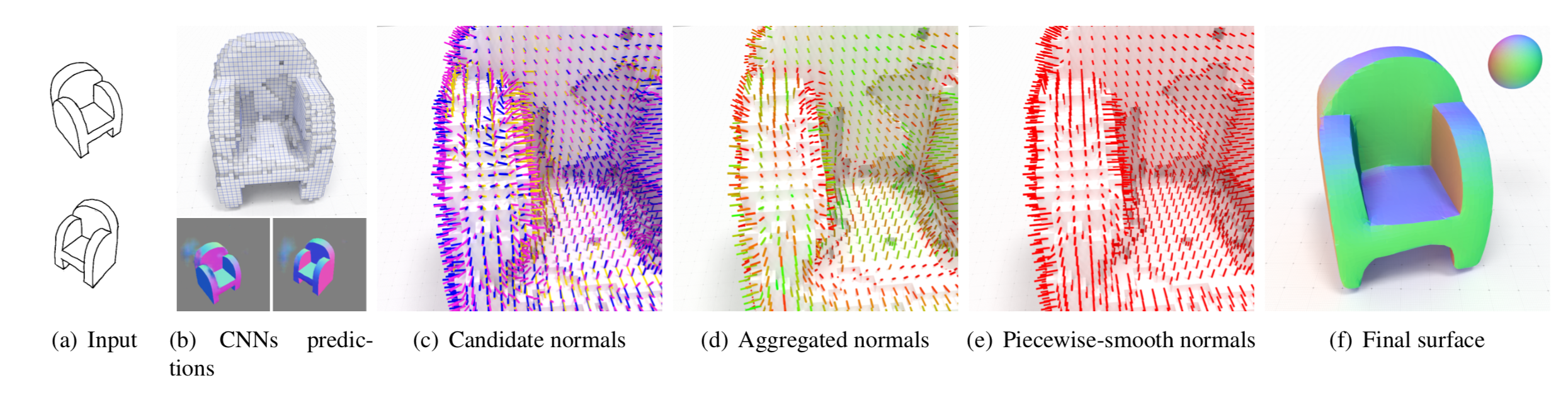
Combining Voxel and Normal Predictions for Multi-View 3D Sketching Johanna Delanoy, David Coeurjolly, Jacques-Olivier Lachaud, Adrien Bousseau. Computers and Graphics, 82:65–72, 2019
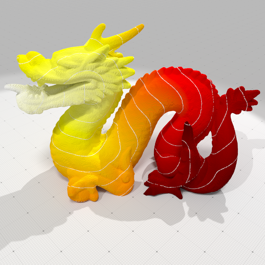
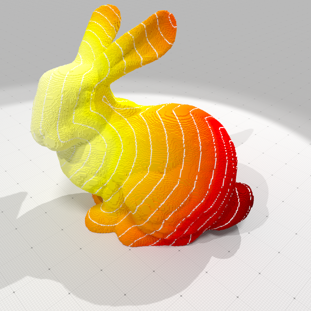
Regularized surface as a smooth proxy
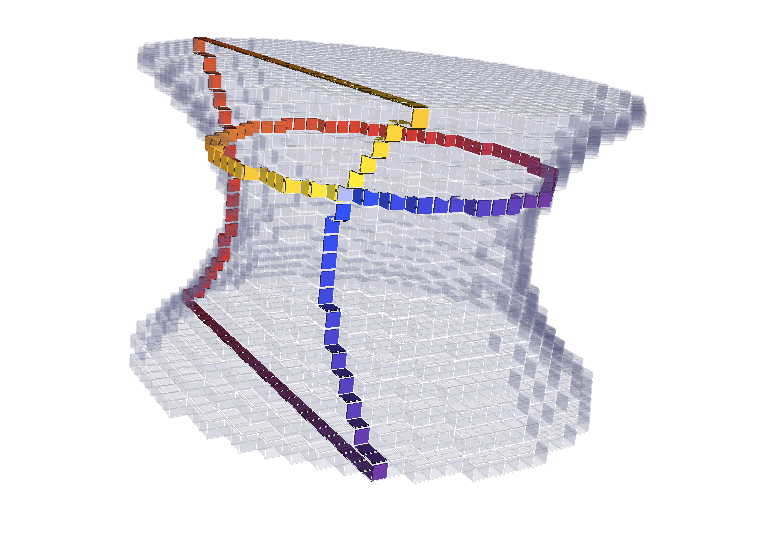
Curvature estimation
Integral Invariant approach: integration ball centers are projected onto the regularized surface.
 |  |
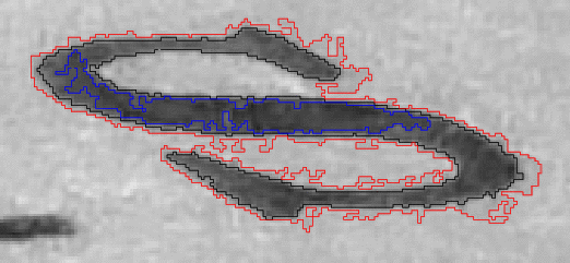
Subpixel Euclidean distance transformation
Separable Distance Transformation + [Lindblad, J., Sladoje, N., 2015]
 |  |
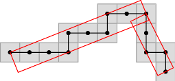
Multigrid convergent pixel/voxel coverage estimation
$\Rightarrow$ Key ingredient in many quantity estimation applications
- Using the regularized proxy: still $O(h^2)$ worst-case error in the coverage estimation :/, much lower error in practice
- E.g. projecting on maximal straight lines (2D) : $O(h^{7/3})$ (Conj.)

DGtal Packages
$$\tiny \mathbb{Z}^d $$ 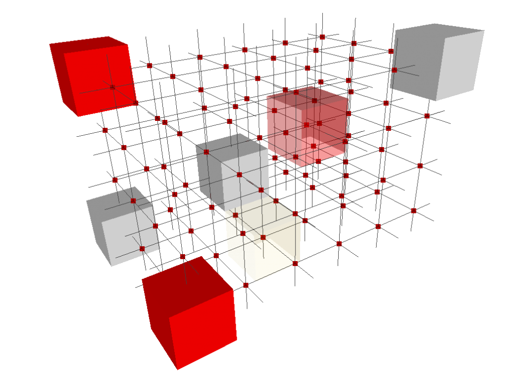 |
$$\tiny u_0+\frac{1}{u_1+\frac{1}{\ldots+\frac{1}{u_k}}} $$ 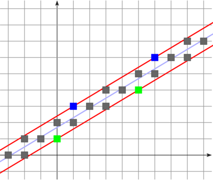 |
  |
  |
  |
| Kernel | Arithmetic | Geometry | Shapes | Topology |
|---|---|---|---|---|
 |
 |
$$Ax=b$$  |
 |
  |
| DEC | Graph | Mathematic | Image | IO |
Conclusion
- Nice geometrical model with many interactions (arithmetic's, theory of words, computational geometry, discrete mathematics...)
- Very specific discrete/continuous properties
- Related to various areas (image processing, material sciences, geometrical modeling, rendering...) data
- Multigrid convergent framework
- for discrete-continuous
- to validate estimators: length, surface area, coverage, volumetric integrals, curvature tensor, Laplace-Beltrami on surfaces...
- Discrete Exterior Calculus on digital surfaces with intrinsic metric information