Point Sampling in Monte Carlo Rendering
Context
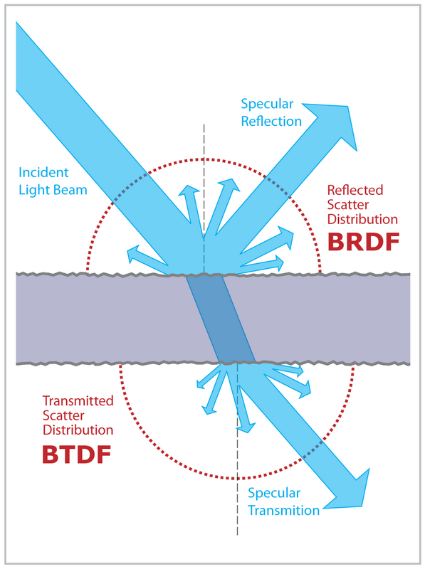
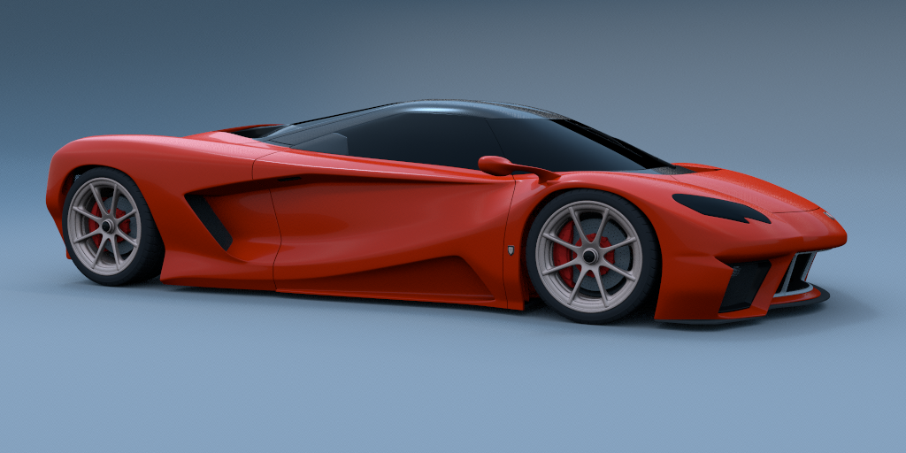
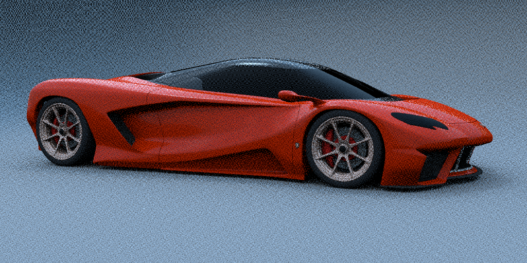
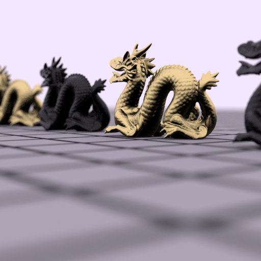
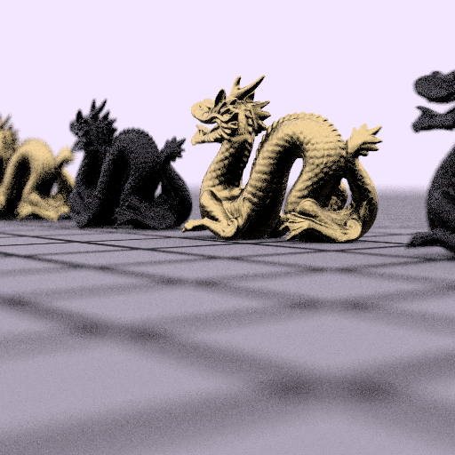
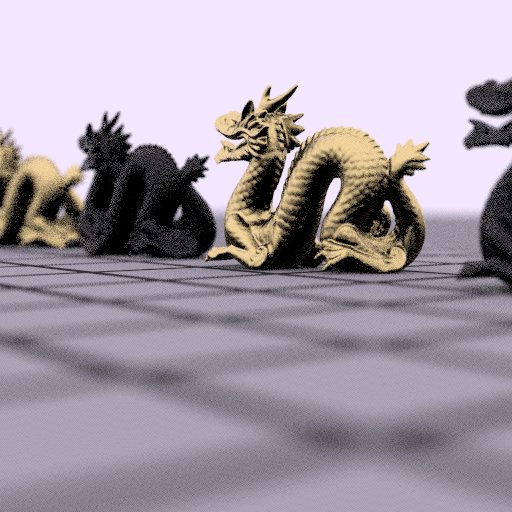
Image rendering: simulate light transport
[Kaj76] $$\mathcal{I}(\vx) = L_e(\vx) + \int_\mathcal{H} \rho(\vp, \vx) \mathcal{I}(\vp) d\vp$$

Numerical approximation
Monte Carlo Estimation
$$\int_D f(x)dx \approx \frac{1}{n} \sum_{i=0}^{n} f(x_i)$$

Monte Carlo Estimation
$$\int_D f(x)dx \approx \frac{1}{n} \sum_{i=0}^{n} f(x_i)$$

Monte Carlo Estimation
$$\int_D f(x)dx \approx \frac{1}{n} \sum_{i=0}^{n} f(x_i)$$

Material Design
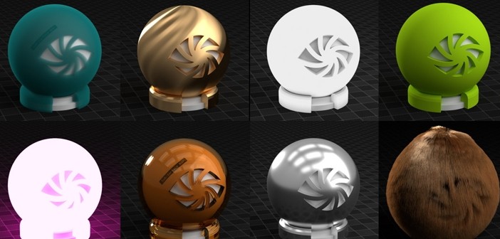
We need samples in n-D
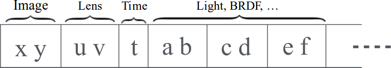
Many strategies
- for path construction (bidirectional, gradient domain...)
- to sample the n-D space (adaptive, importance sampling, multiple importance sampling...)
- to correlate samples from one pixel to a neighboring one
- to post-filter/reconstruct the final image
- ...
We need fast samplers
Error, Bias, Variance
$\mathcal{I} = \int_\Omega fdx$
$\mathcal{I}_n = \frac{1}{n}\sum f(x_i), \quad \{x_i\}\in \Omega$
$$ \Delta := | \mathcal{I} -\mathcal{I}_n | $$
$$ \langle \Delta\rangle := \mathcal{I} - \langle \mathcal{I}_n \rangle $$
$$ \text{Var}(\mathcal{I}_n) := \langle \mathcal{I}_n^2 \rangle - \langle \mathcal{I}_n \rangle^2 $$
Convergence speed


Four main classes

 [Shi91]
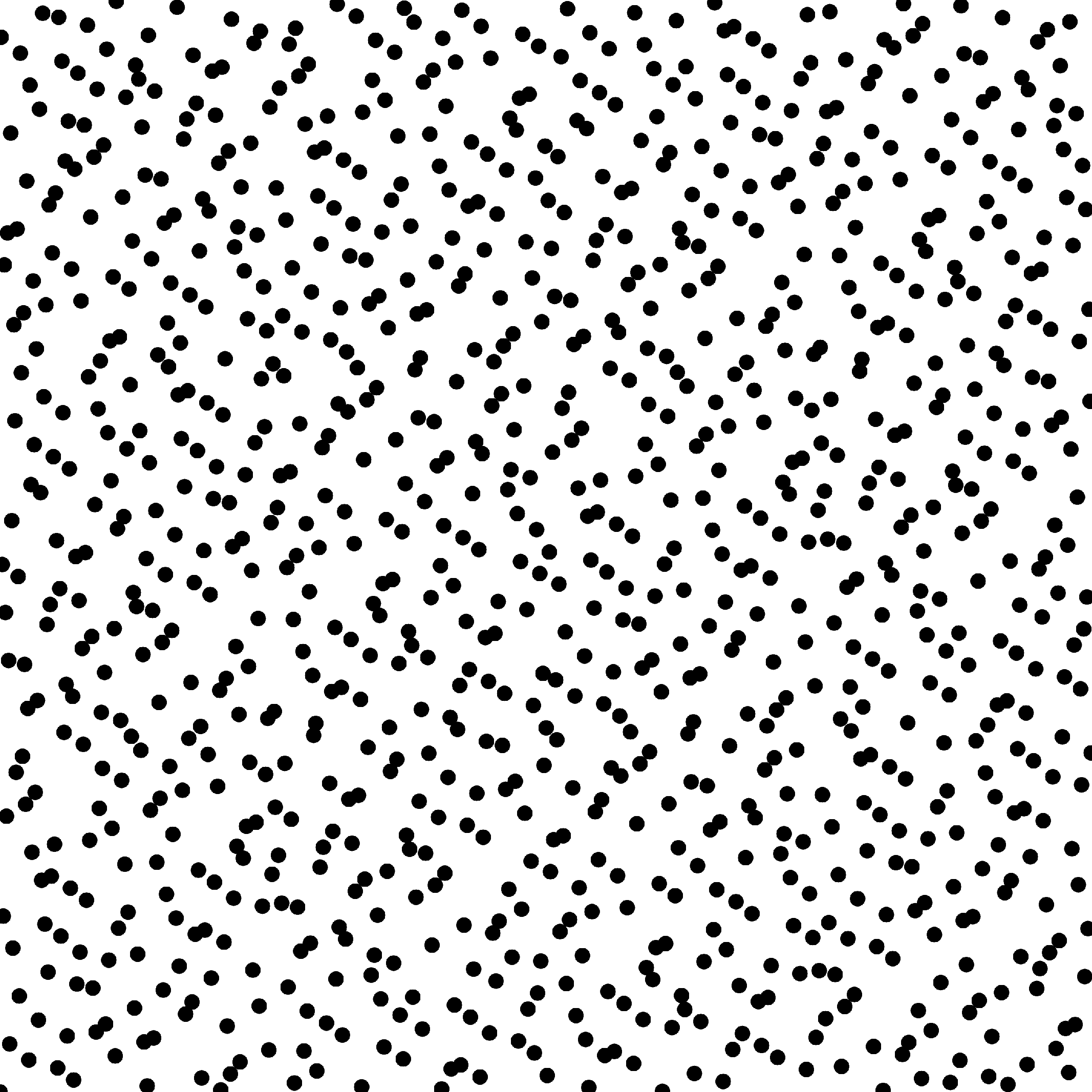
 [Hal64]
[HH64]
[Sob67]
[Hal64]
[HH64]
[Sob67]

 [Coo96]
[Bri07]
[MF92]
[Coo96]
[Bri07]
[MF92]

 [GBO+12]
[CYK+12]
[Fat11]
[GBO+12]
[CYK+12]
[Fat11]
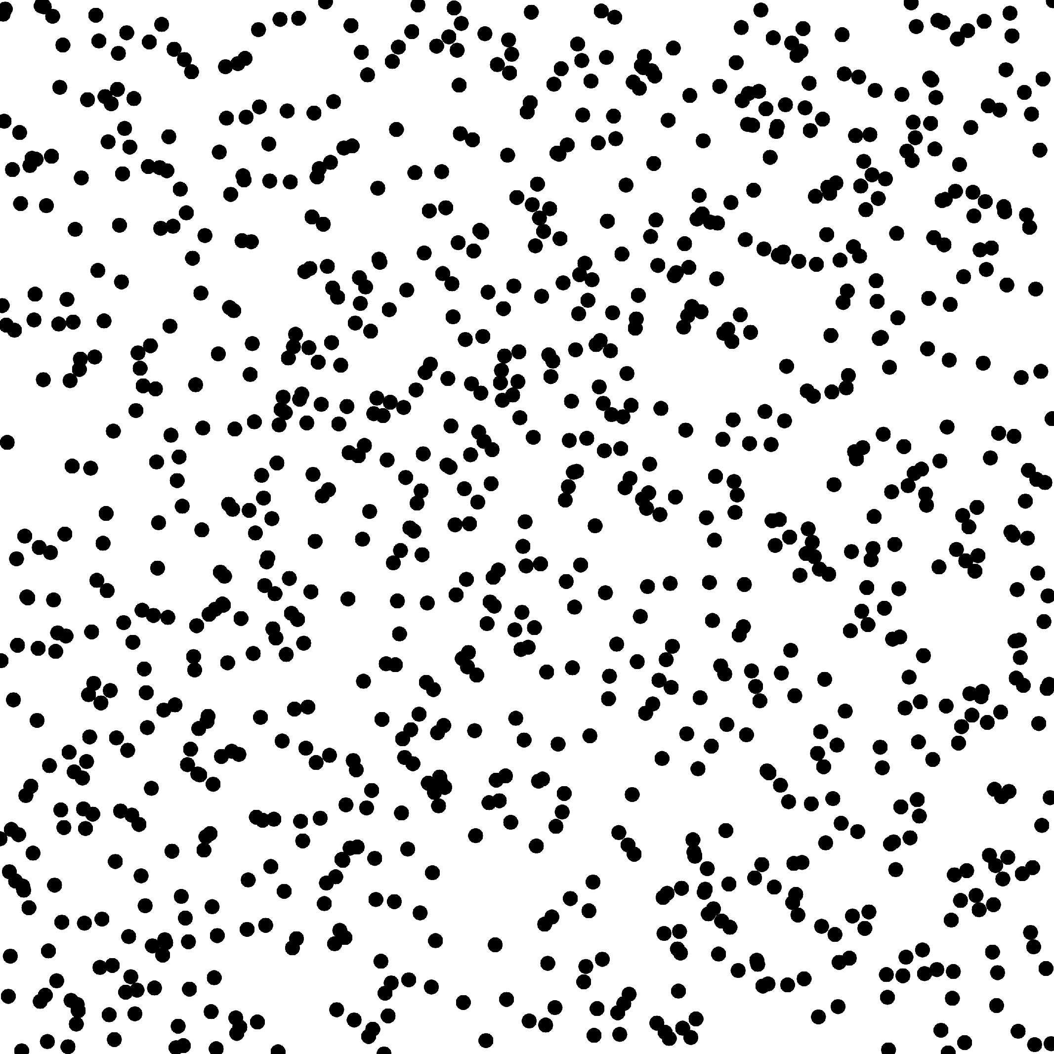
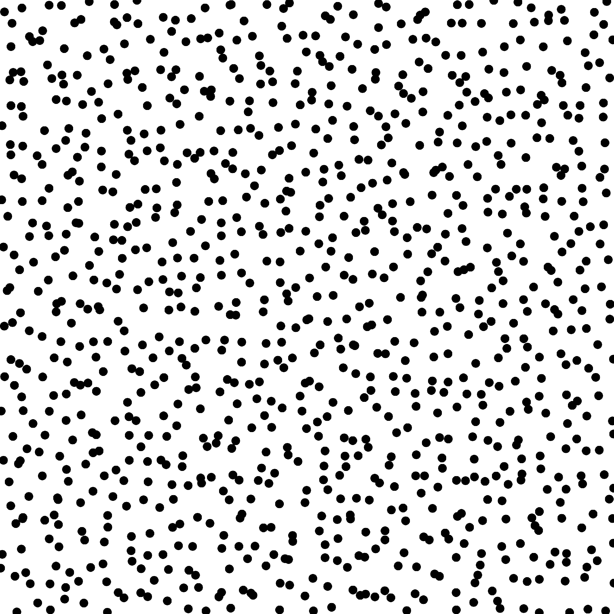
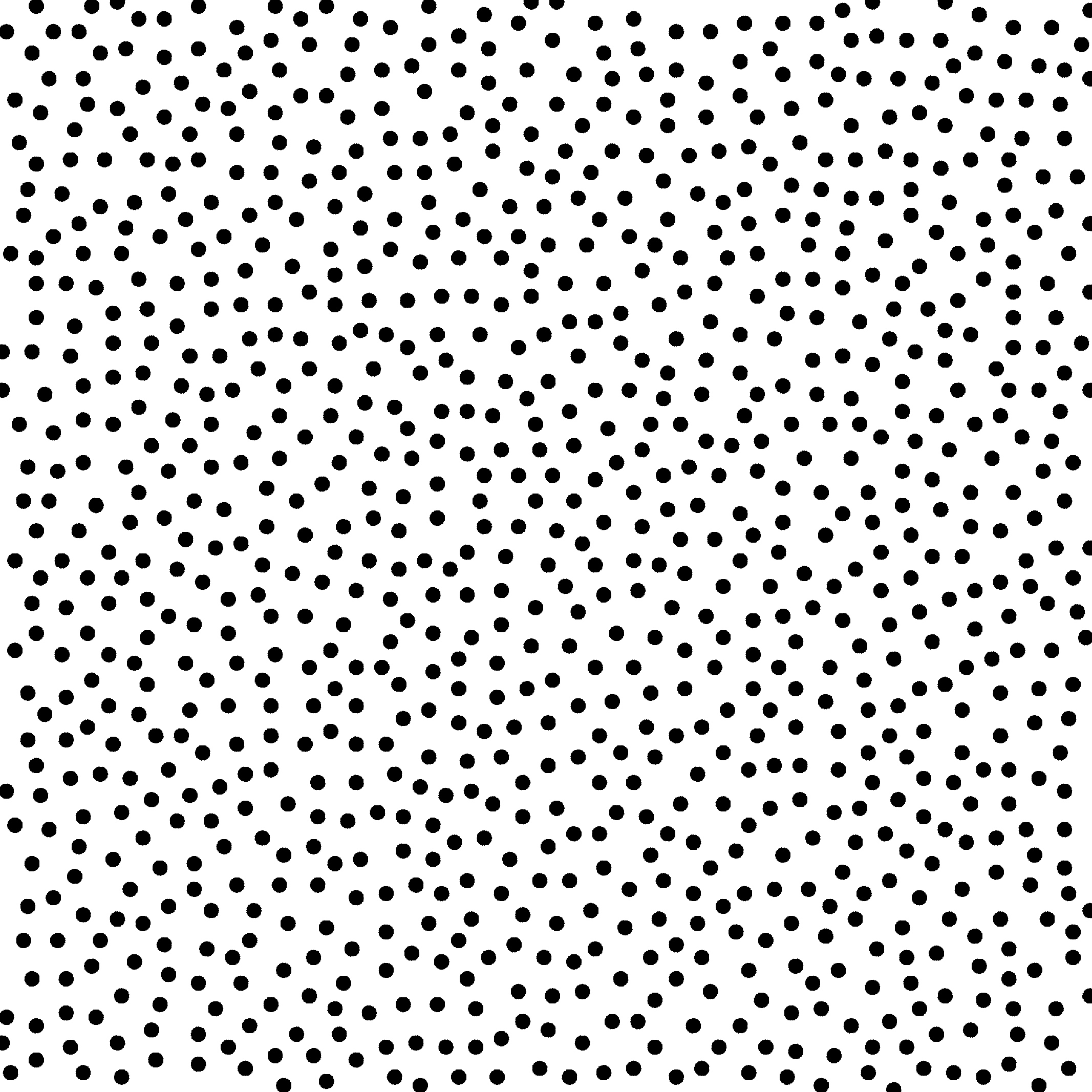
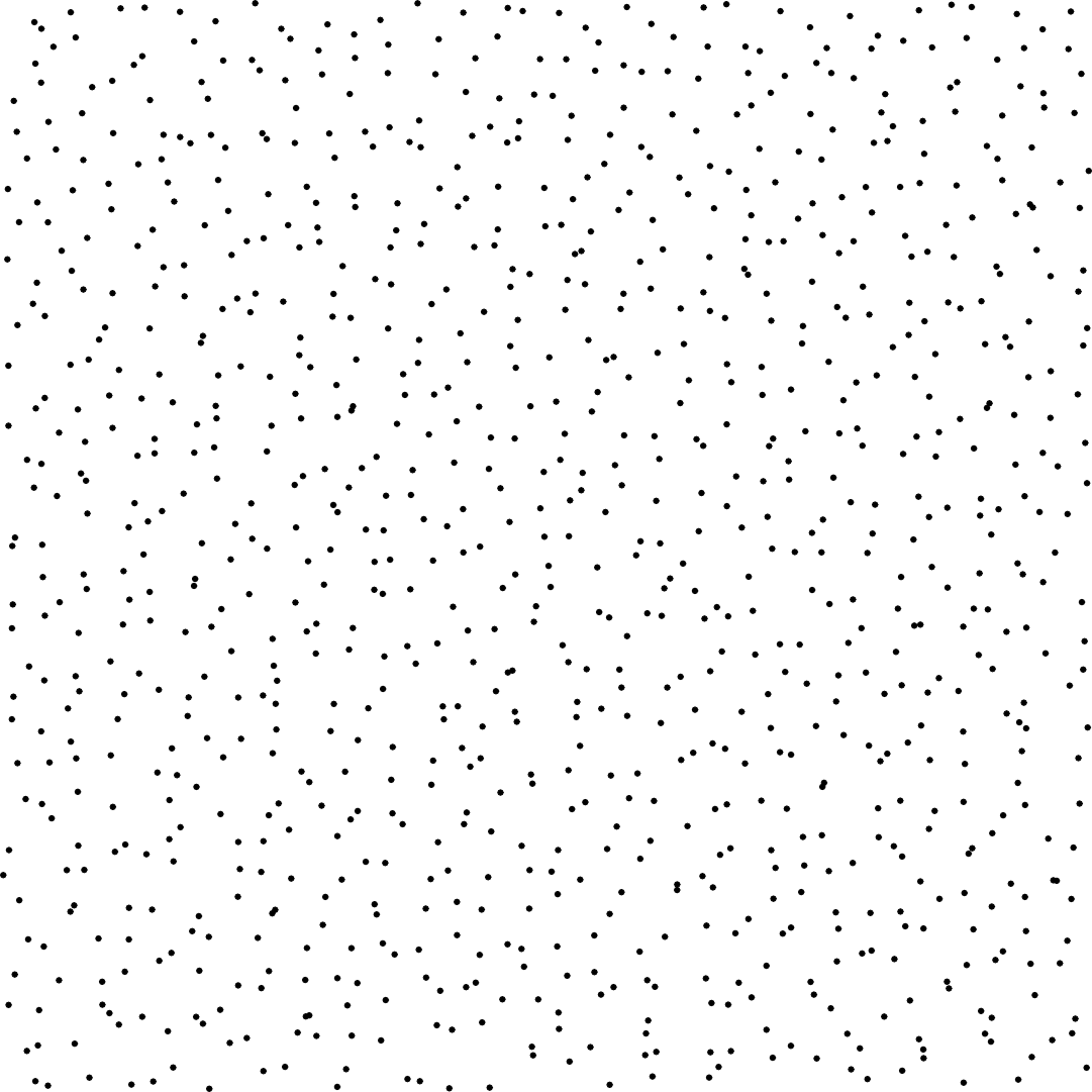
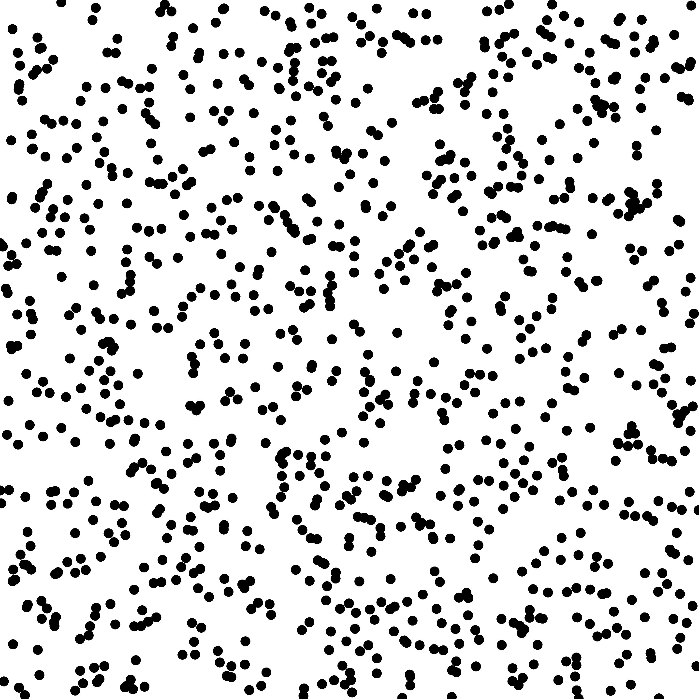
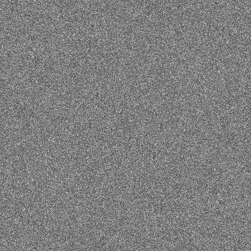
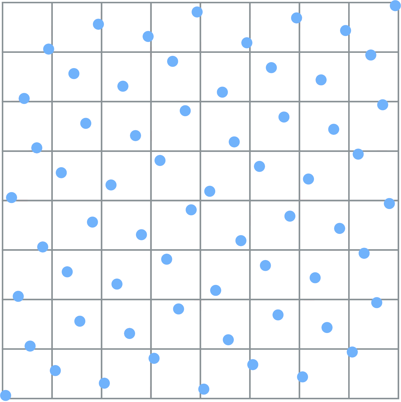
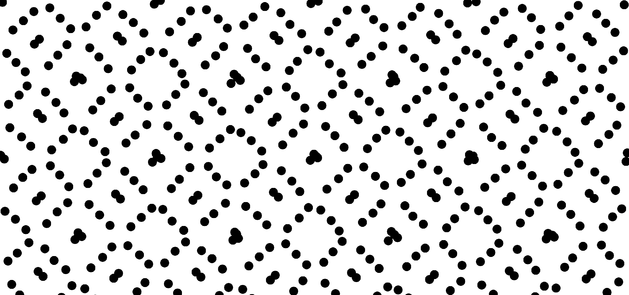
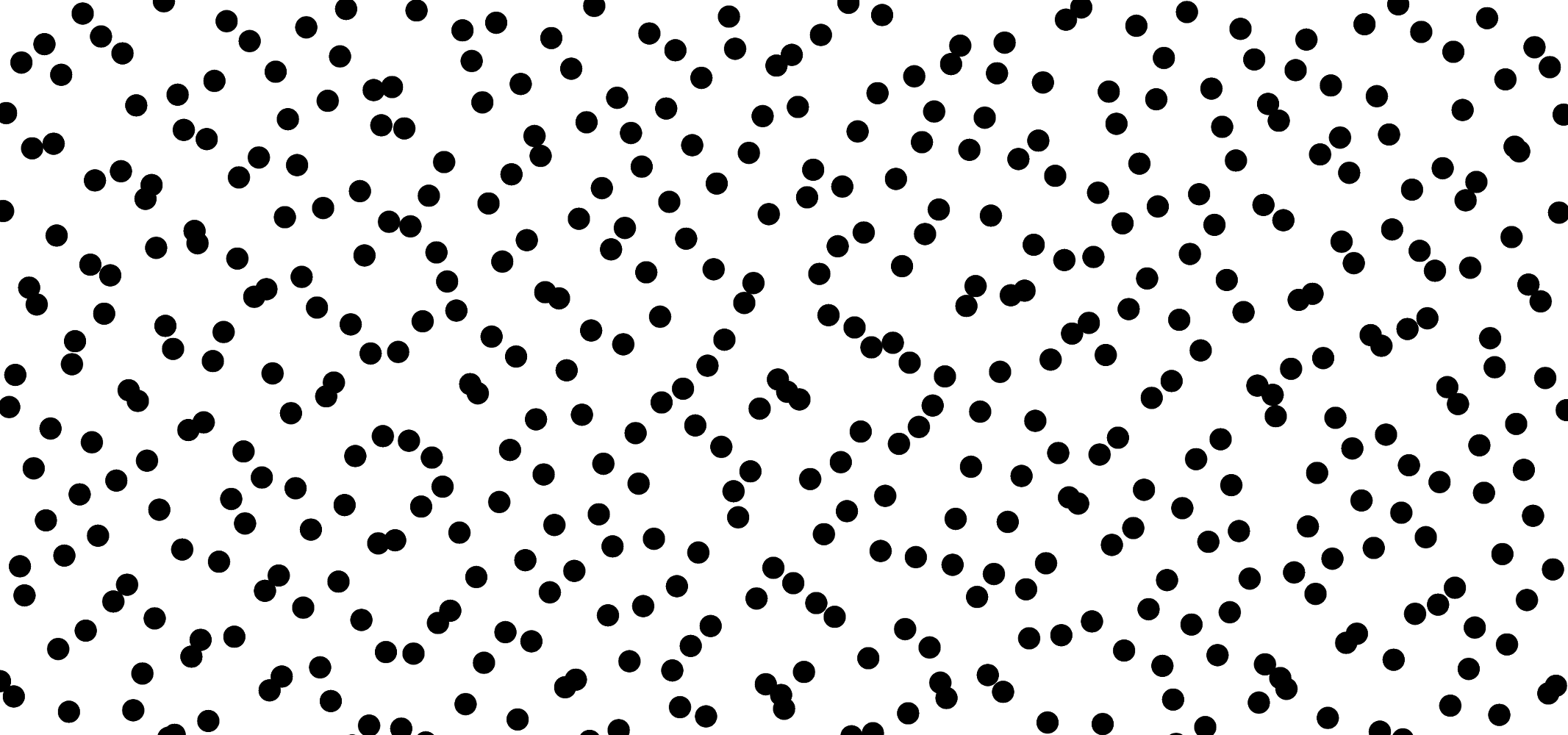
Whitenoise / Poisson process
$$ Var(I_n) = O\left(\frac{\sigma_f^2}{{n}}\right) $$
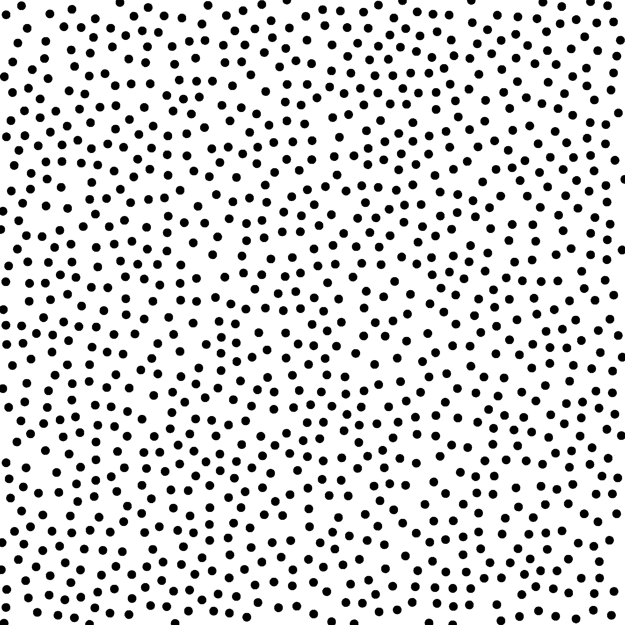
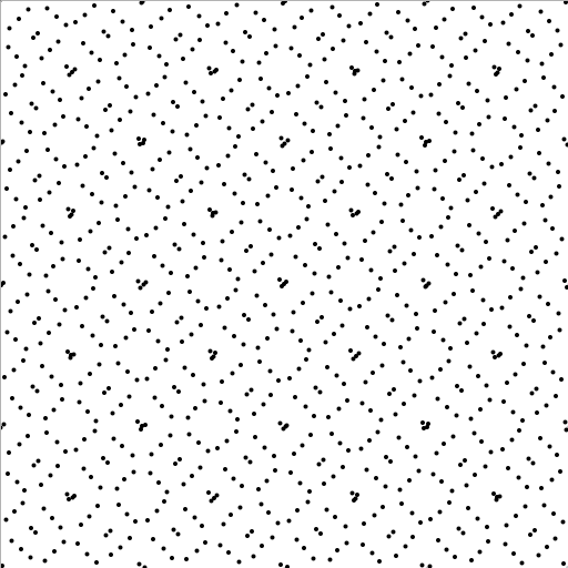
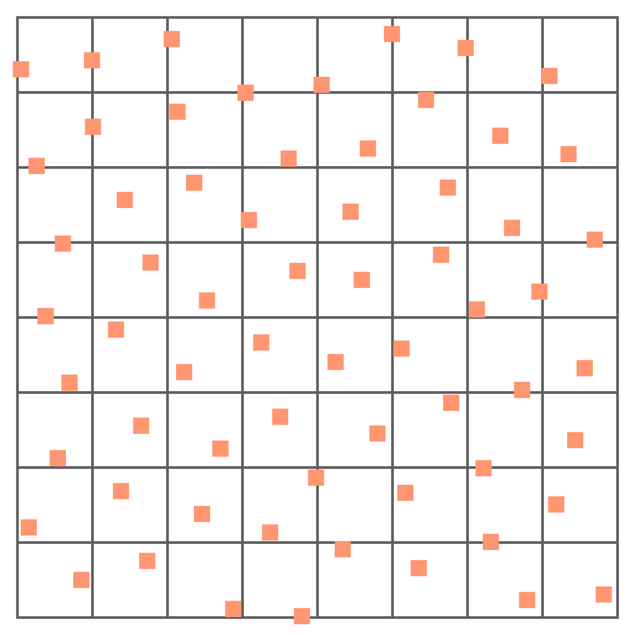
Poisson disk / Dart throwing
Higher quality for low sample counts but... $$ Var(I_n) = O\left(\frac{1}{{n}}\right) $$ {demo}
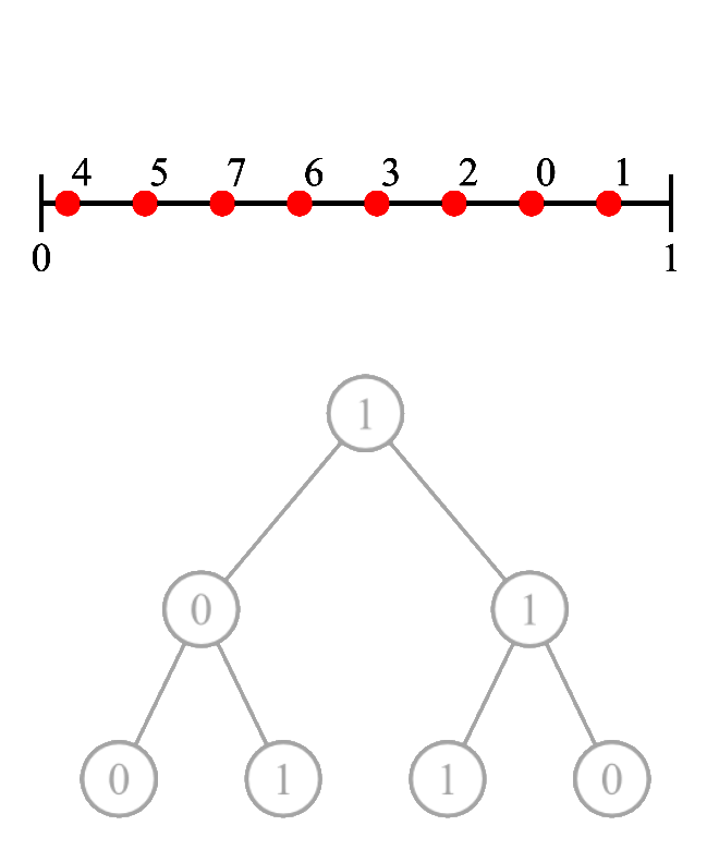
van der Corput 1d Sequences (whiteboard)
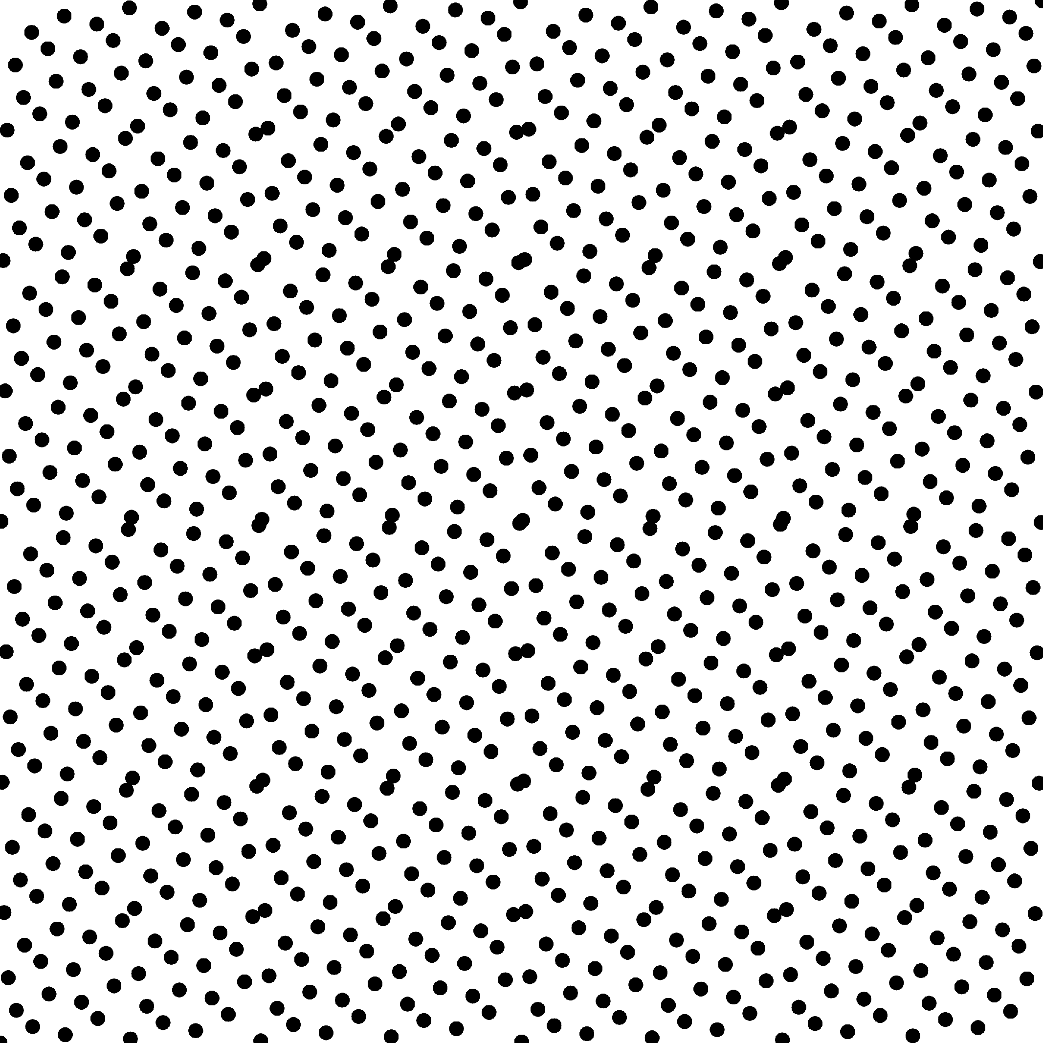
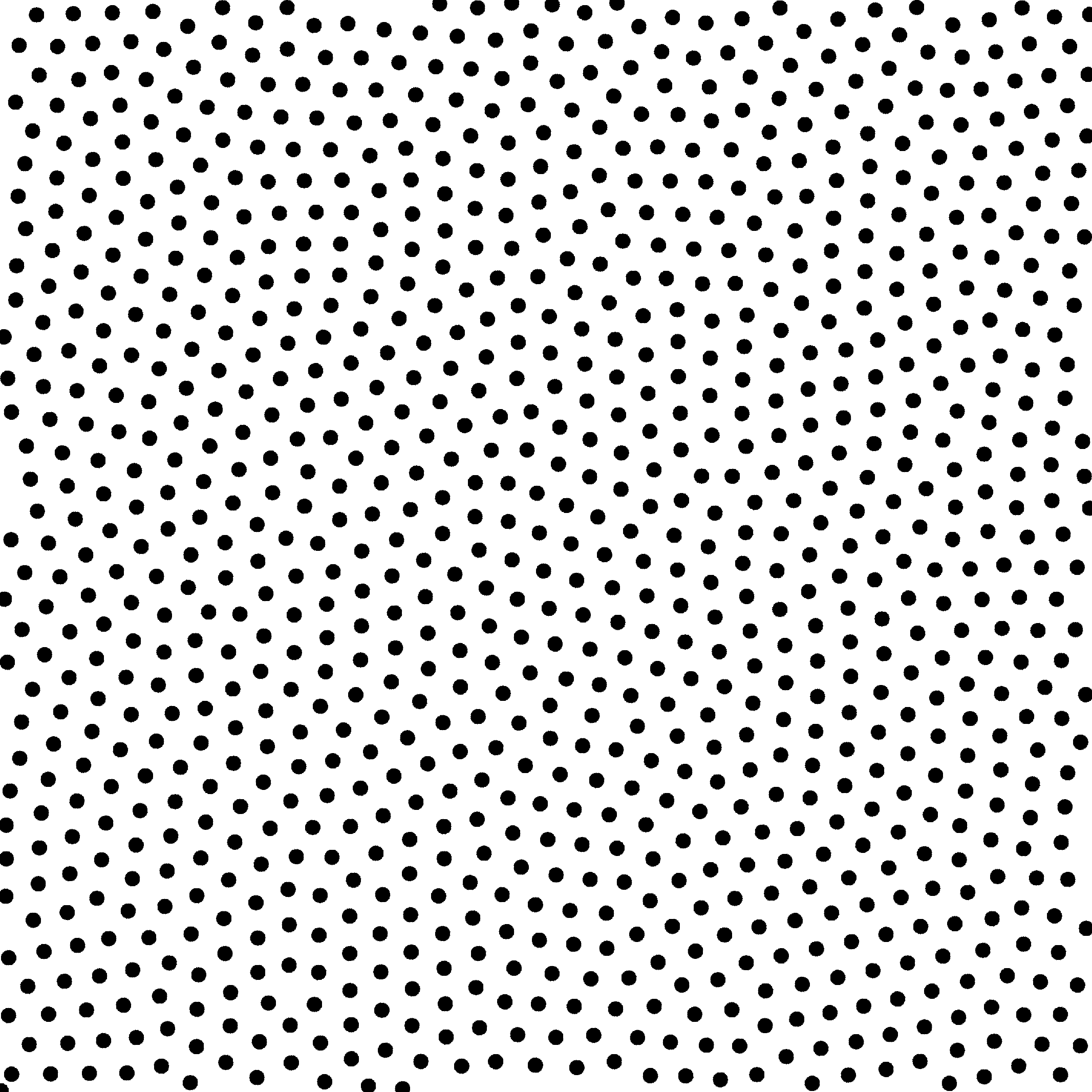
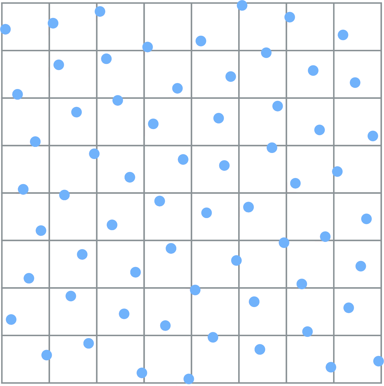
Low discrepancy sequences / Halton
|
E.g.: $x(n)=(g_{{b_{1}}}(n),\dots ,g_{{b_{s}}}(n))$ in dimension $s$
and $b_1,\ldots,b_{s-1}$ arbitrary coprime integers $g_{b}(n)=\sum _{{k=0}}^{{L-1}}d_{k}(n)b^{{-k-1}}.$ (b-ary representation of the positive integer expressed in fractional part) |
$$ \Delta = O\left(\frac{ \log(n)^{d-1}}{n}\right) $$ {demo}
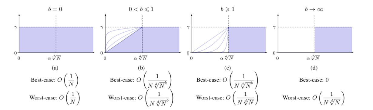
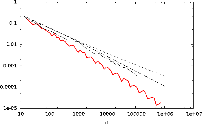
Few convergence speeds
$$
Var(I_n) = O\left(\frac{\sigma_f^2}{{n}}\right)
$$
$$
\Delta = O\left(\frac{
\log(n)^{d-1}}{n}\right)
$$
$$
Var(I_n) = O\left(\frac{1}{n\sqrt[d]{n}} \right)
$$
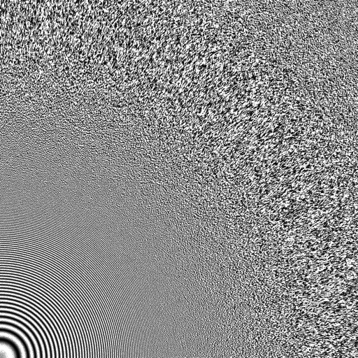
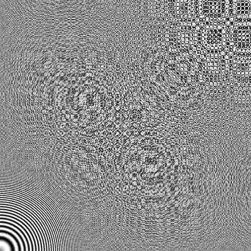
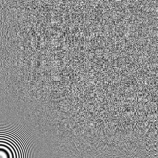
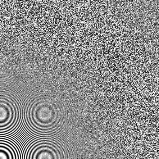
Aliasing and error structure
Aliasing and error structure

Aliasing and error structure
Wrap-up
Sampling process:
- Uniform in $[0,1)^d$
- With asymptotic bounds on the variance reduction for MC / QMC
- Stochastic processes but with correlation between samples
Image rendering context:
- Reatively limited number of dimensions (~30/40)
- As few as possible structure (aliasing)
- As efficient as possible even for low sample count
- Fast and progressive sampler
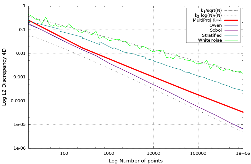
Evaluation tools
Discrepancy
Evaluate the uniformity of a point set $P_n$
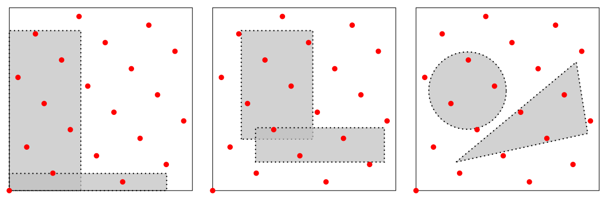
| Star discrepancy |
Extreme discrepancy | Isotropic discrepancy |
$f$ is an Hardy & Krause bounded variation function.
Discrepancy
A sampler is low discrepancy if its discrepancy is in $O\left(\frac{\log(n)^{d-1}}{n}\right)$.
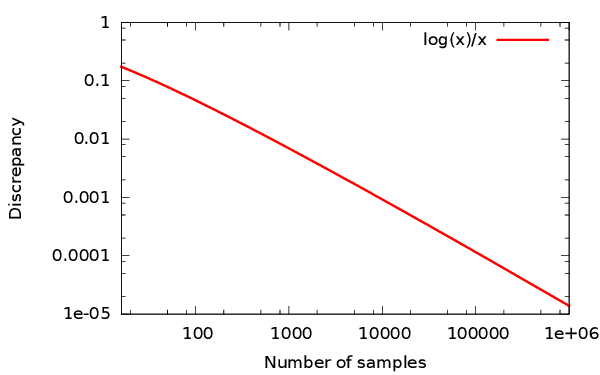
$$ \Delta = O\left(\frac{ \log(n)^{d-1}}{n}\right) $$ (for finite HK-BV integrand compared to $O(1/\sqrt{n})$ for Poisson sampler)
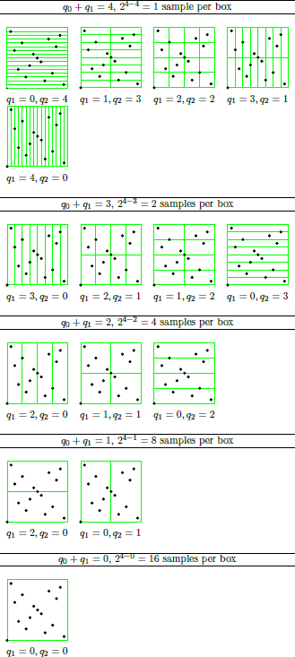
QMC sampler examples
E.g. $i=11 = (1011)_2$, $\phi(i)=(.1101)_2 = \frac{1}{2} + \frac{1}{4} + \frac{1}{16} = 0.8125 \in[0,1)$

arithmetic on $\mathbb{Z}/p\mathbb{Z}$...
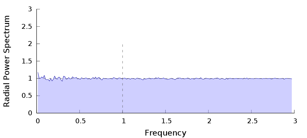
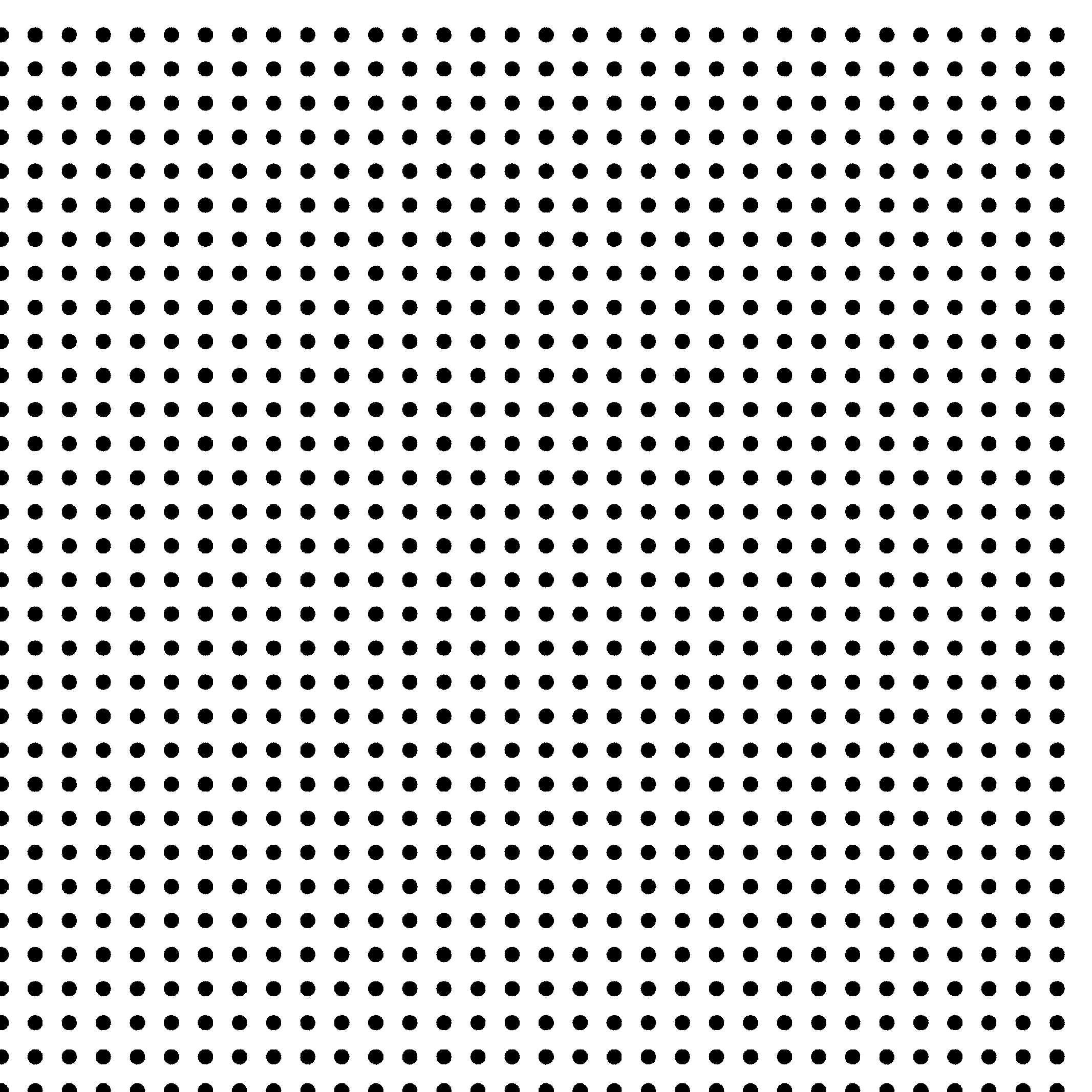
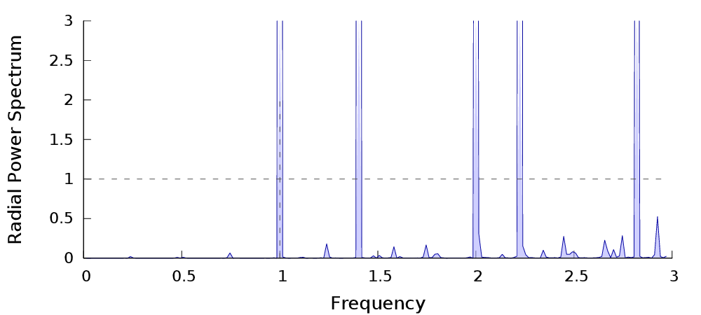
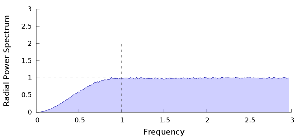
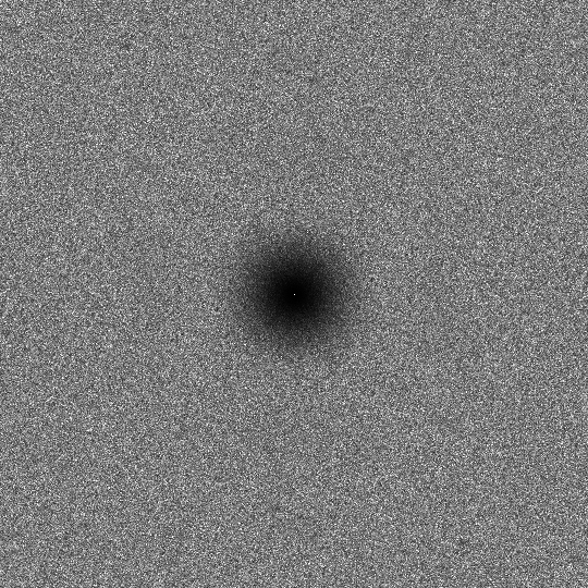
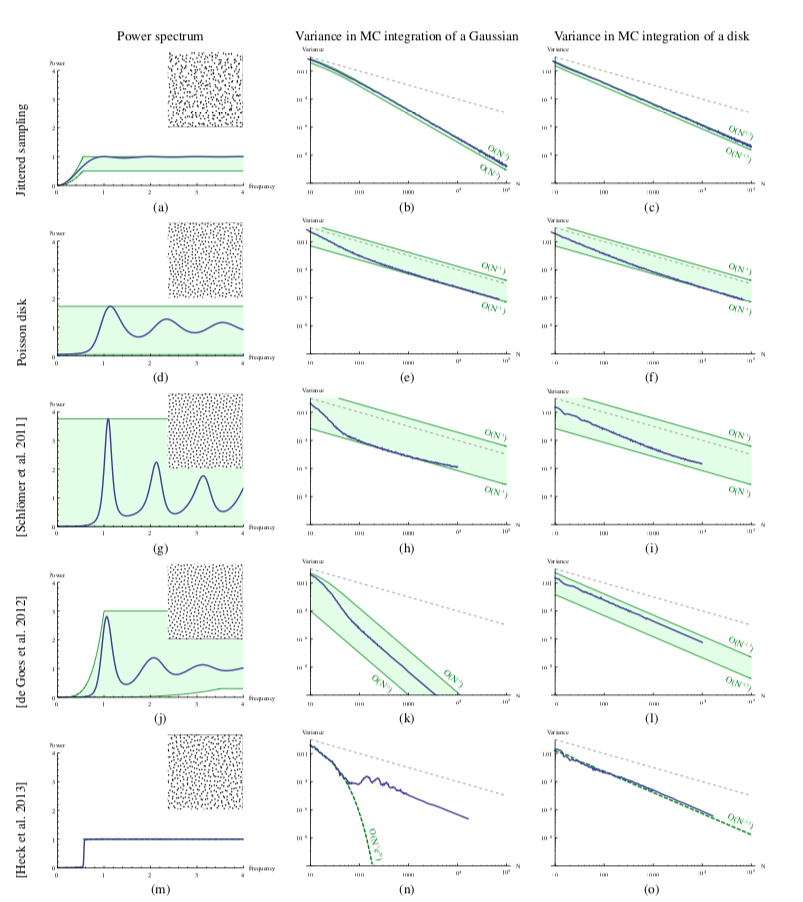
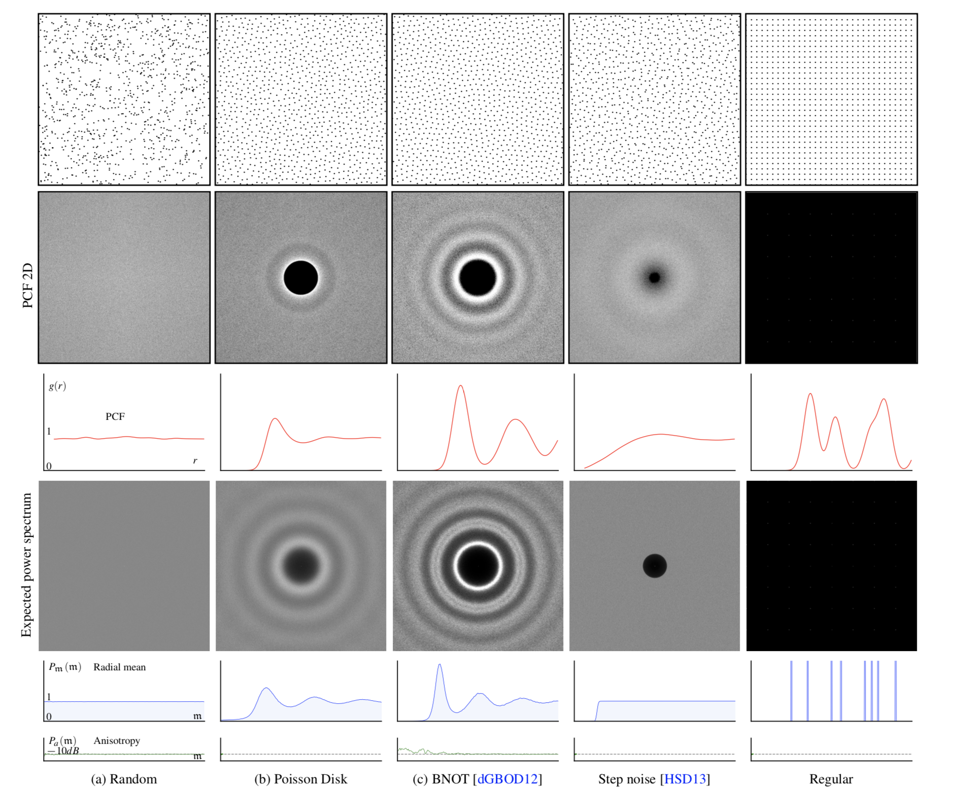
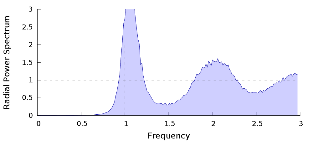
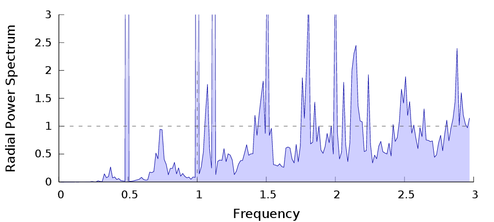
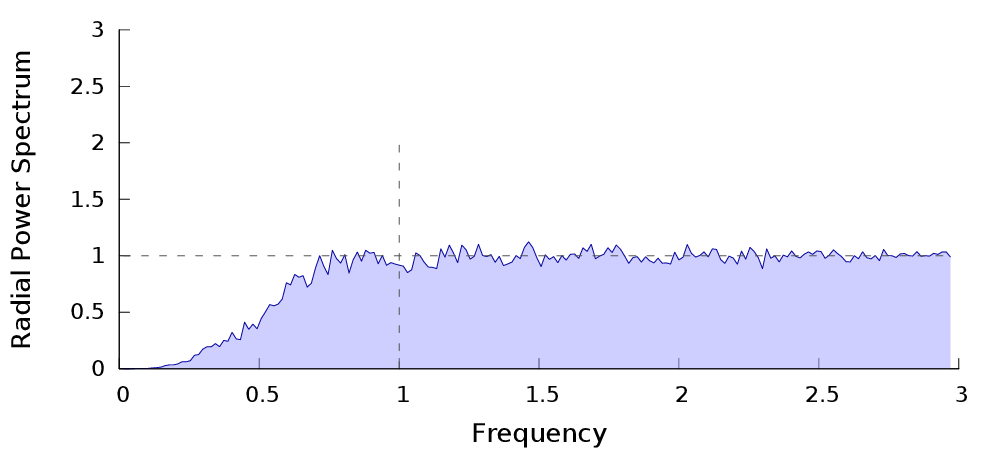
Spectral Analysis
| $P_n$ | Power spectrum� | Radial Power Spectrum |


Spectral Analysis
|
|
 |
|
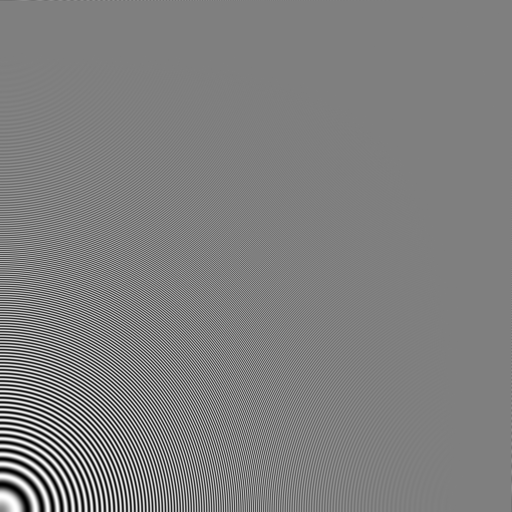
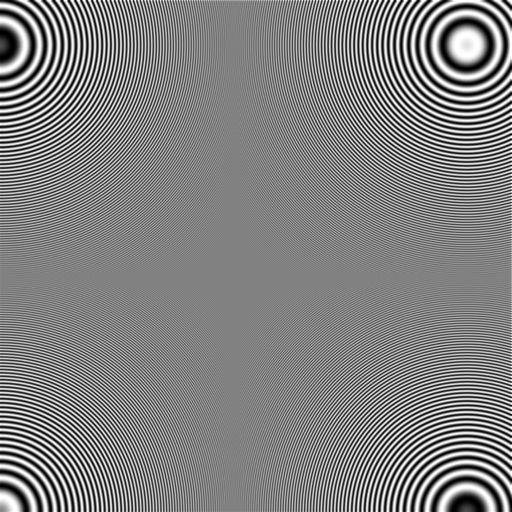
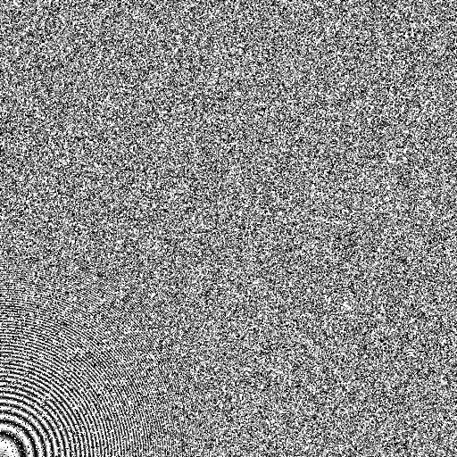
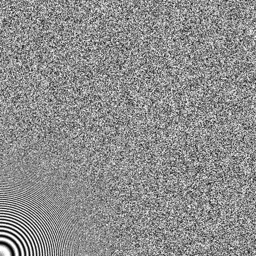
| $sin(x^2 + y^2)$ |  |
 |
 |
 |
 |
 |
 |
Analysis
$$S(x) = \frac{1}{n}\sum_{k=1}^n \alpha_k \delta(x-x_k)\quad \text{and its $m$-th Fourier series coefficient}\quad \mathbf{S}_m = \frac{1}{n}\sum_{k=1}^n \alpha_k e^{-i2\pi m x_k}\,,$$ we have $$\mathcal{I}_n=\int_0^1 f(x)S(x)dx = \int_\mathbb{R} \mathcal{F}_f(v)\mathcal{F}_S(v)dv =\sum_{m=-\infty}^{\infty} \mathbf{f}_m^* \mathbf{S}_m$$
If $S(x)$ is a stochastic point process:
$$\langle \Delta \rangle = \mathbf{f}_{0}^*(1 - \langle
\mathbf{S}_0\rangle) - \sum_{m\in\mathbb{Z}, m\neq 0}
\mathbf{f}_m^*\langle \mathbf{S}_m\rangle$$
$$Var({I}_n) =
\mathbf{f}_0^*\mathbf{f}_0 Var(\mathbf{S}_0)
+ \sum_{m\in\mathbb{Z}, m\neq 0}\mathbf{f}_m^*\mathbf{f}_m\langle
\mathbf{S}_m^*\mathbf{S}_m\rangle + \sum_{m \in
\mathbb{Z}}\sum_{l \in \mathbb{Z}, l\neq m}
\mathbf{f}_m^*\mathbf{f}_l\langle
\mathbf{S}_m^*\mathbf{S}_l\rangle$$
$\langle \Delta \rangle =
\mathbf{f}_{0}^* - \sum_{m\in\mathbb{Z}, m\neq 0}
\mathbf{f}_m^*\langle \mathbf{S}_m\rangle$
$\langle \Delta
\rangle = 0$ for Poisson process (or any unbiased sampler)
$Var({I}_n) =\sum_{m\in\mathbb{Z}}\mathbf{f}_m^*\mathbf{f}_m\langle \mathbf{S}_m^*\mathbf{S}_m\rangle$
Spectral Analysis
$Var({I}_n) =\sum_{m\in\mathbb{Z}}\mathbf{f}_m^*\mathbf{f}_m\langle \mathbf{S}_m^*\mathbf{S}_m\rangle$
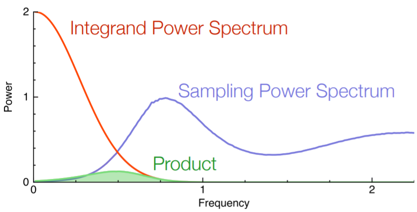
Spectral Analysis
$Var({I}_n) =\sum_{m\in\mathbb{Z}}\mathbf{f}_m^*\mathbf{f}_m\langle \mathbf{S}_m^*\mathbf{S}_m\rangle$
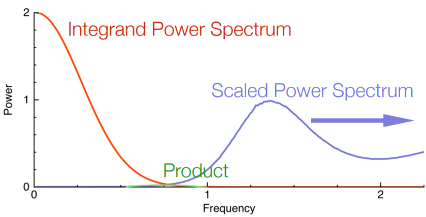
High variance reduction = low energy in the low frequency domain of the sampler
Optimal Transport
Distance between a discrete measure (point pattern = set of Diracs) and a measur (e.g. Uniform measure).
$\Rightarrow$ cf SOT
Related characterizations
Pair Correlation Function, Differential Analysis...
Few convergence speeds
$$
Var(I_n) = O\left(\frac{\sigma_f^2}{{n}}\right)
$$
$$
\Delta^2 = O\left(\frac{
\log(n)^{2(d-1)}}{n^2}\right)
$$
$$
Var(I_n) = O\left(\frac{1}{n\sqrt[d]{n}} \right)
$$
The Ideal Sampler in CG
- Uniform in $[0,1)^d$
- With highest asymptotic variance reduction in MC / QMC integration
For rendering:
- Rather limited number of dimensions (~30/40)
- No structure or patterns (for aliasing issues)
- Low error for low sample counts
- Fast sampler and progressivity

Polyhex
Aperiodic tile-based system

- Precomputed samples in a hierarchical tiling system for fast blue noise sampling (+ 1 million samples/sec)
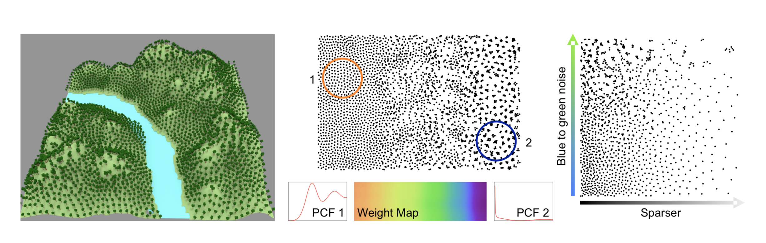
- Local density control
- 2D
- Extremely fast
- High quality blue noise
- Adaptive sampling
- 2D only
- Huge precomputed LUT
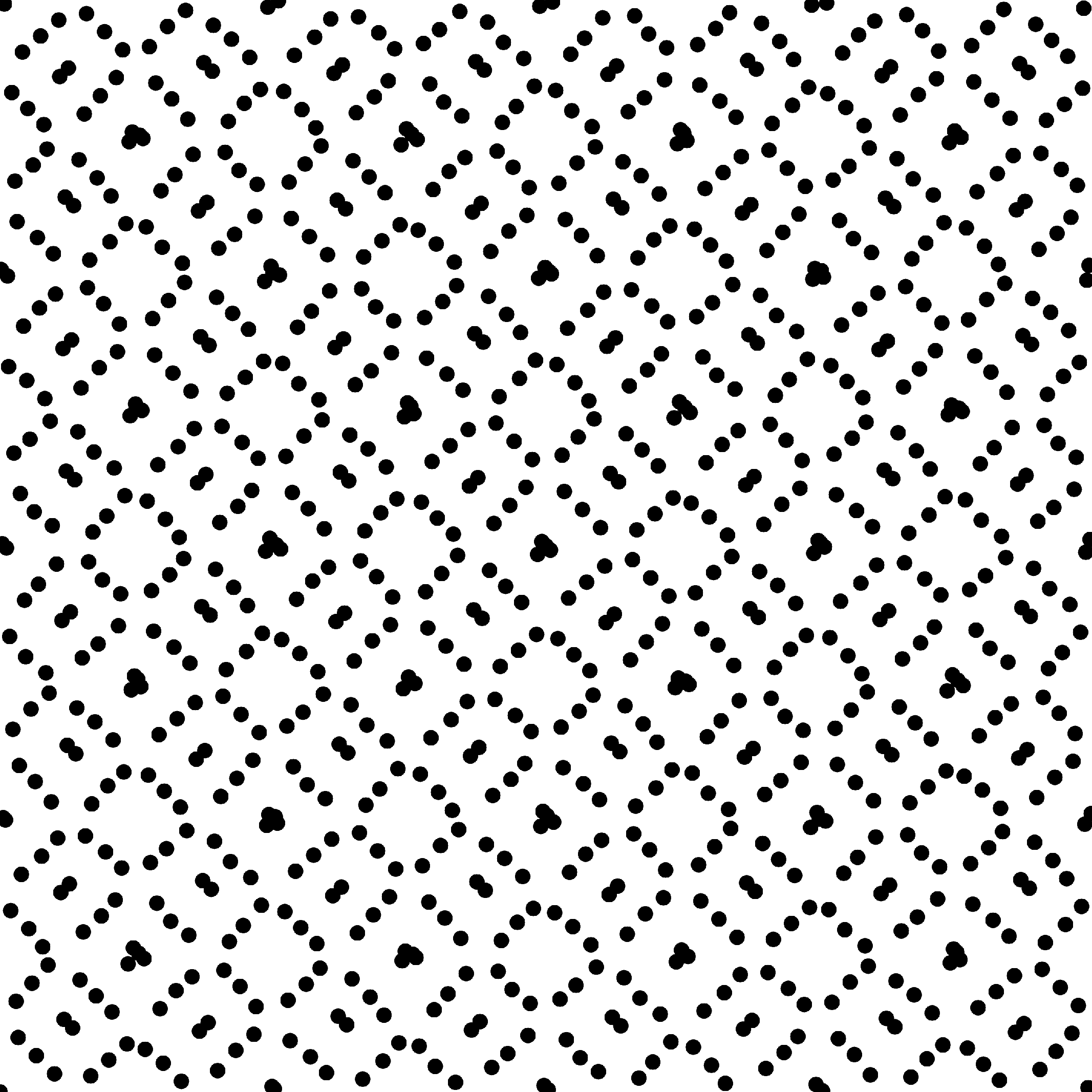
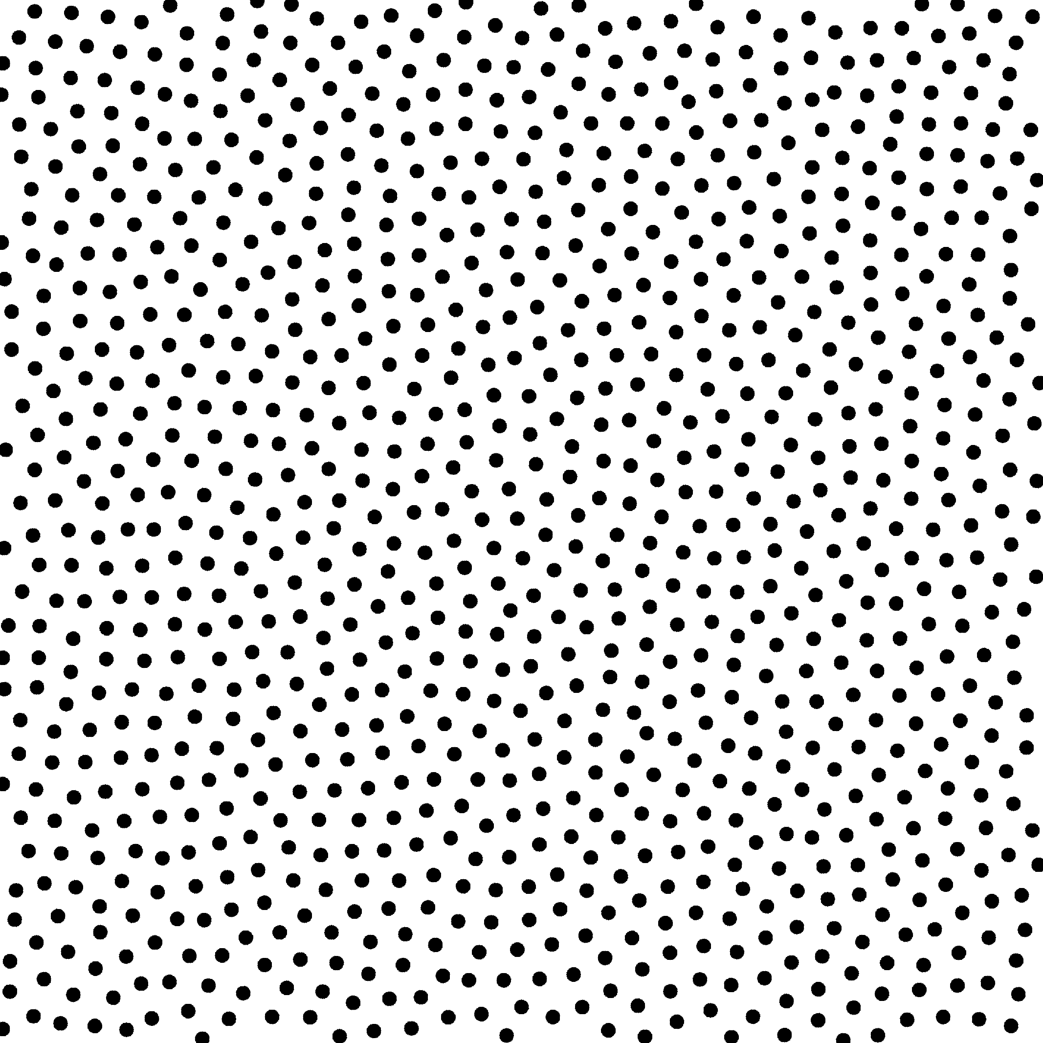
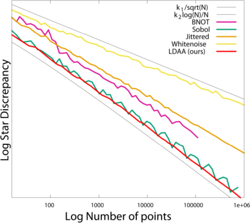
Low Discrepancy Blue Noise
Low discrepancy Blue Noise in 2D
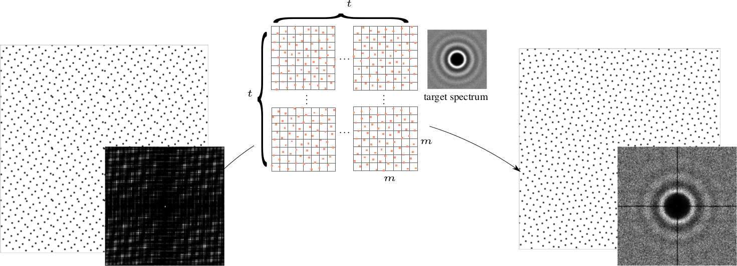
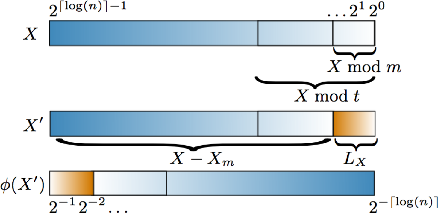
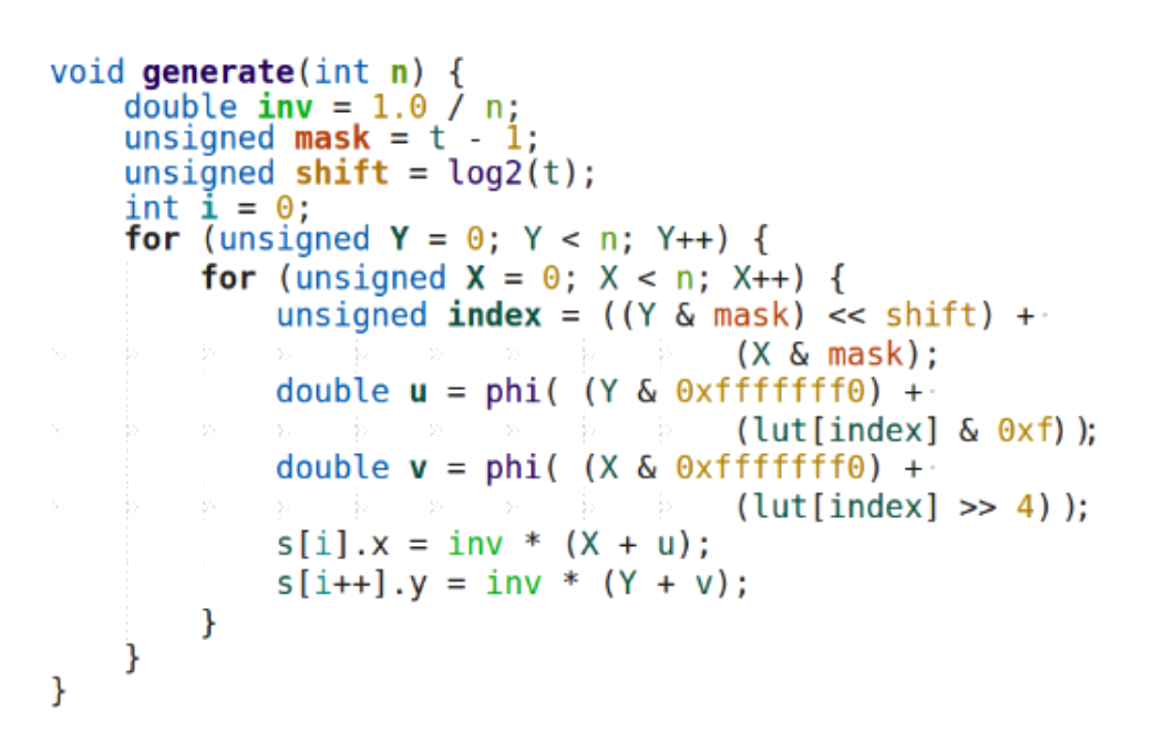
The method
 |

 |
 |
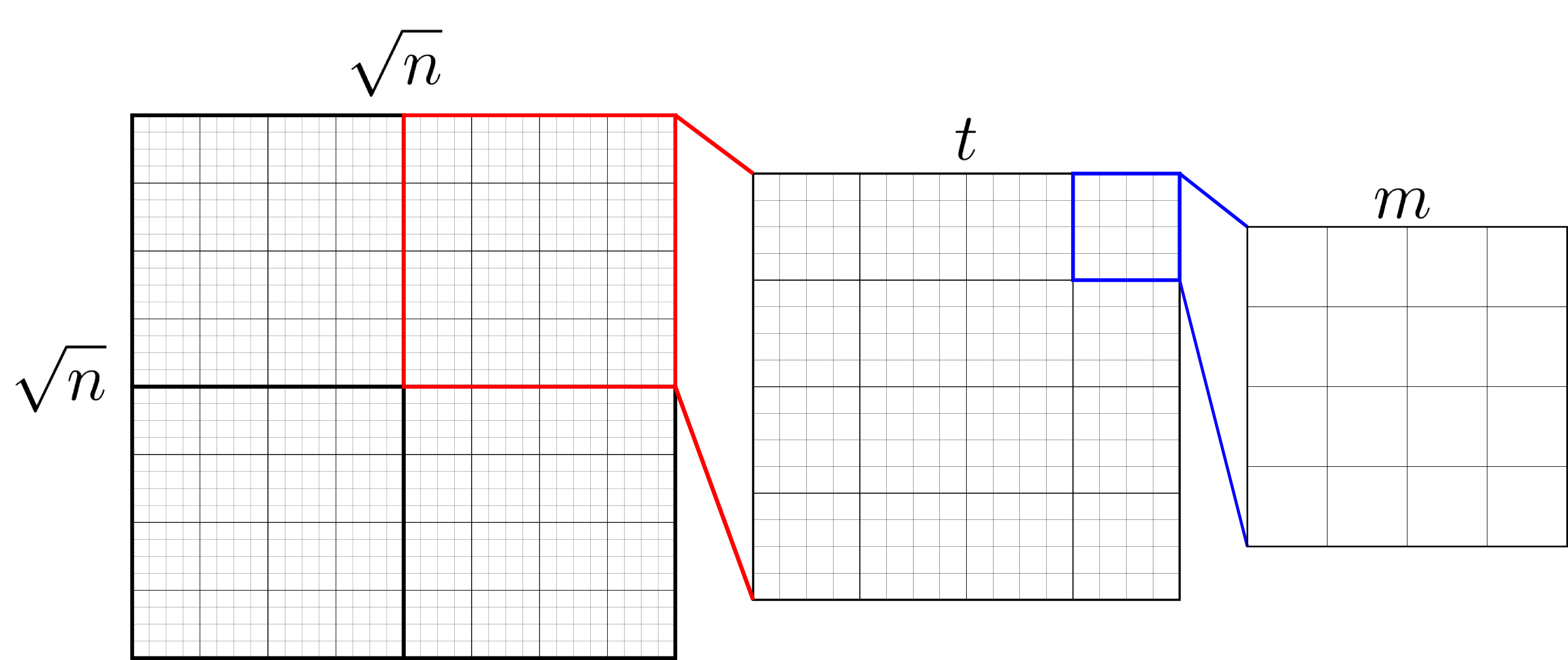
The method
The method
On calcule les permutations de taille $m$ à partir d'un ensemble de taille $t^2$. On les stocke ensuite dans une LUT pour générer des ensembles de taille $n$.
The method
The method
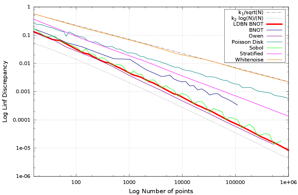
Results
 |
 |
| BNOT [GBO+12] | Sobol [Sob67] |
 |
 |
| Owen's Scrambling [Owe95] | LDBN ($m=16$, $t=128$) |
Results
|
|
| BNOT [GBO+12] | LDBN ($m=16$, $t=128$) |
 |
 |
| Step [HSD13] | LDBN ($m=16$, $t=128$) |
Results
Results
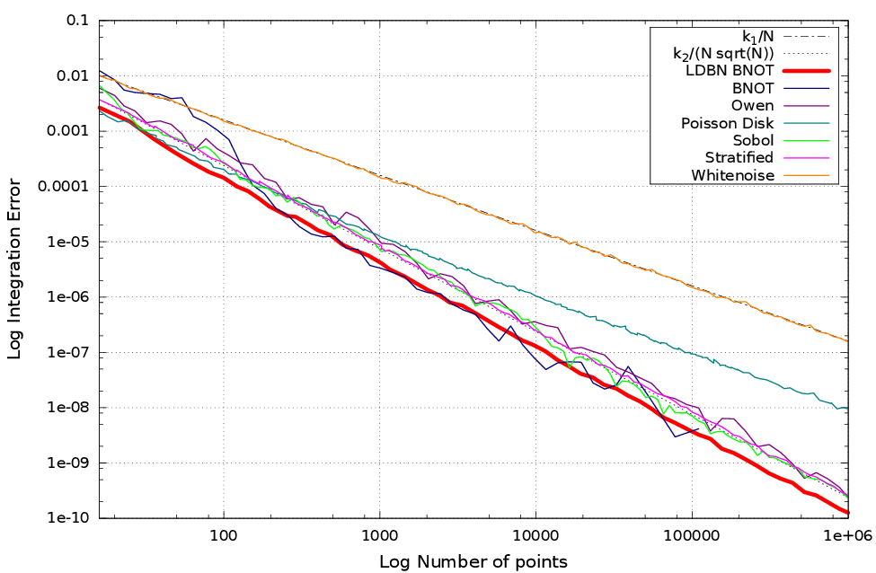
Results
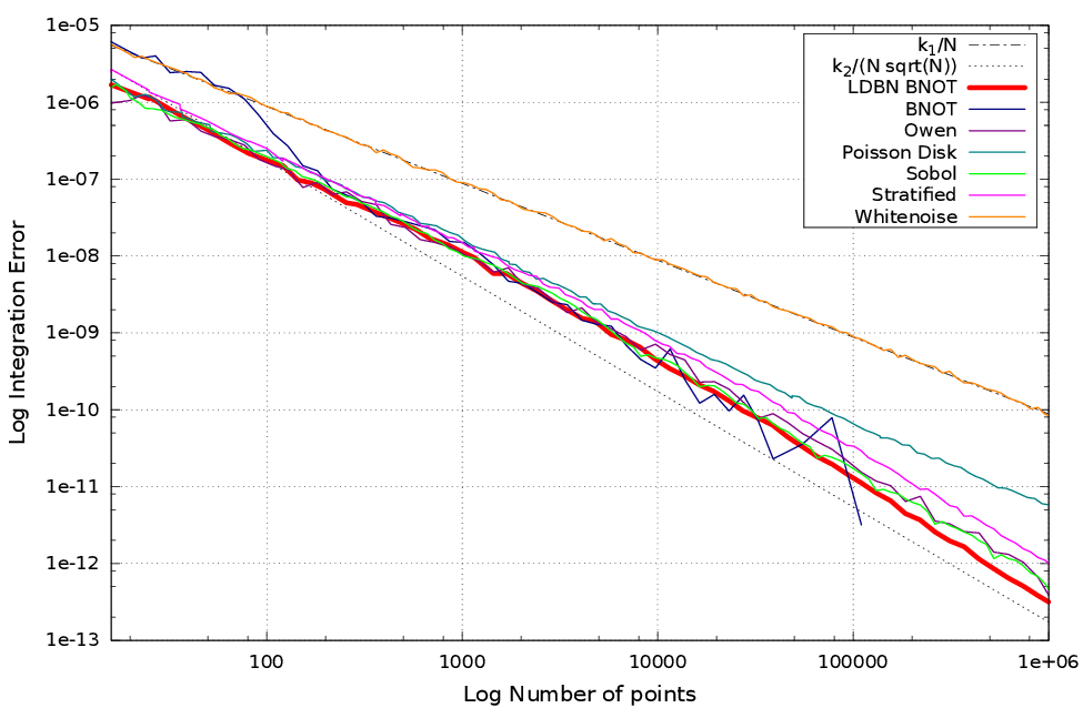
Results

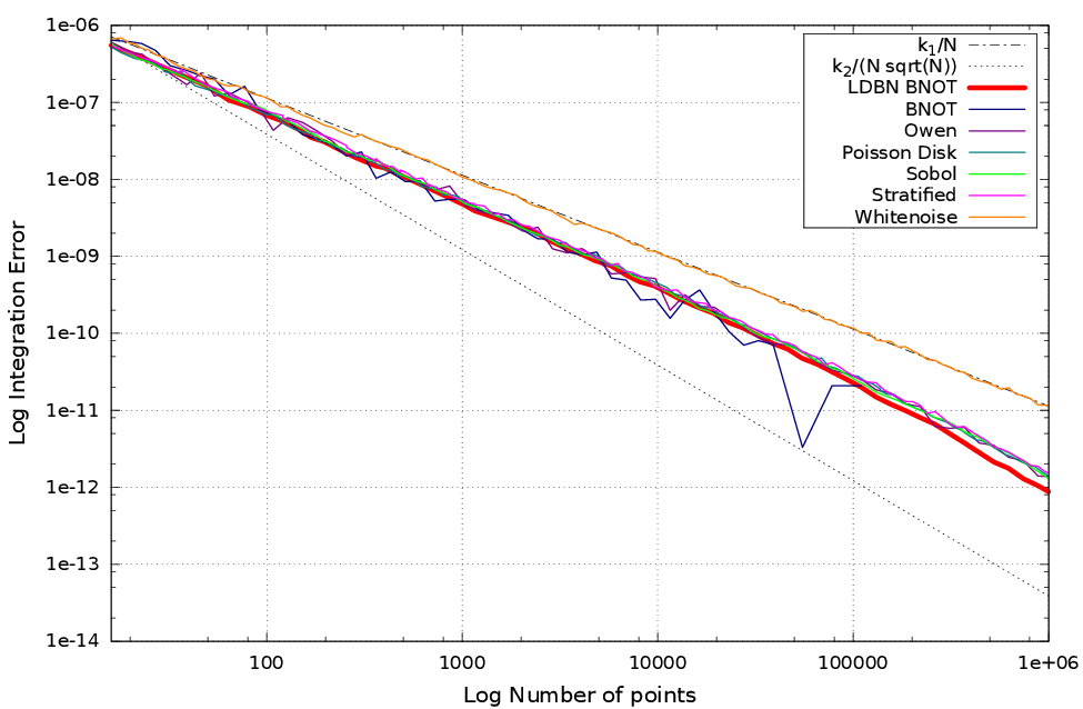
Results

 |
 |
 |
 |
| BNOT [GBO+12] | Sobol [Sob67] | Owen's Scrambling [Owe95] | LDBN ($m=16$, $t=128$) |
- 2D
- Extremely fast
- Very good blue noise distribution
- Low discrepancy point set
- 2D ony
- Not a sequence
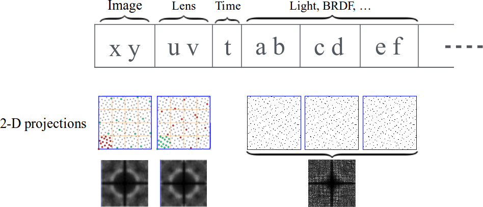
Sequences with Low-Discrepancy Blue-Noise 2-D Projections
Main idea
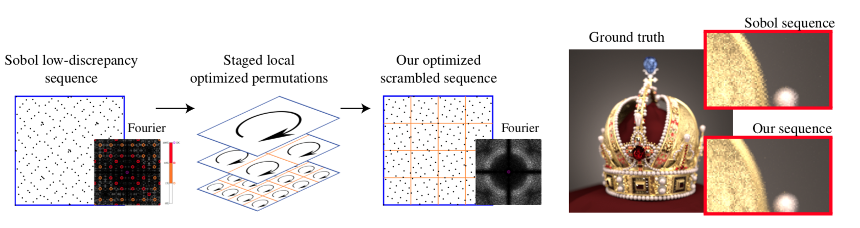
Owen's scrambling [Owe95]
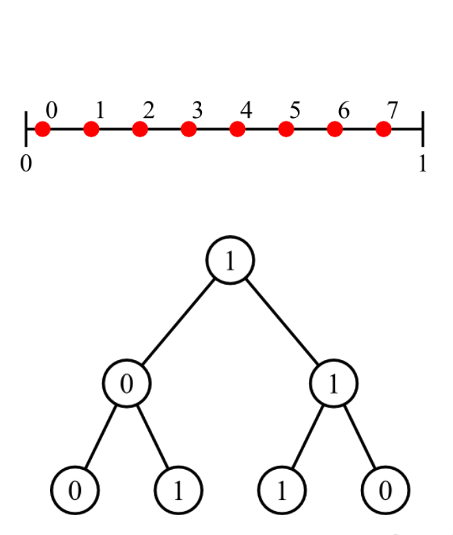
Owen's scrambling [Owe95]
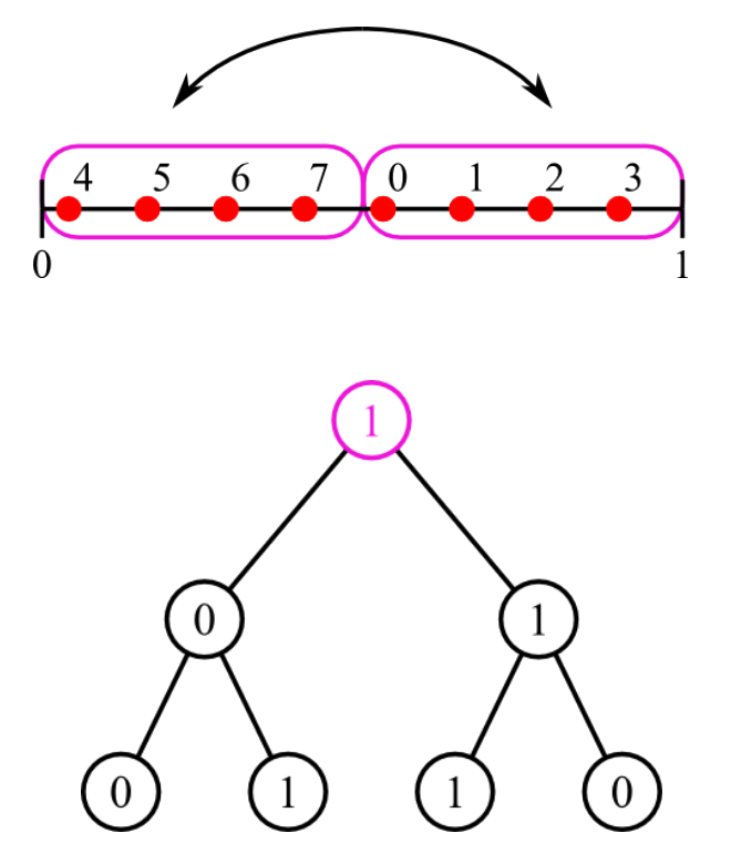
Owen's scrambling [Owe95]

Owen's scrambling [Owe95]
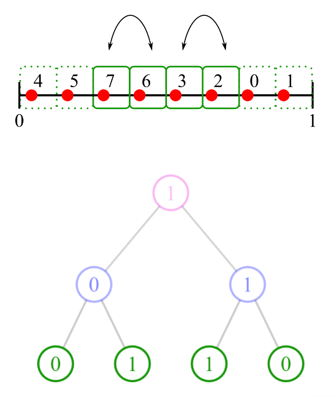
Owen's scrambling [Owe95]
Owen's scrambling [Owe95]


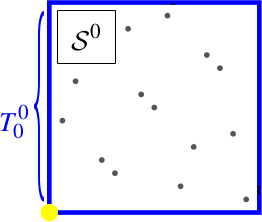
Niveau 1, 2-D, $K=4$
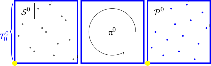
On génère $K^d=16$ points à partir de Sobol. On note cet ensemble $\mathcal{S_0}$.
Et on les mélange en utilisant un Owen scrambling pour leur donner un spectre bruit bleu. On note le nouvel ensemble $\mathcal{P_0}$.
Niveau 2, 2-D, $K=4$
On génère $K^{2d}=256$ points à partir de Sobol. On note cet ensemble $\mathcal{S_1}$.

On commence par appliquer un scrambling global sur cet ensemble pour reconstruire $\mathcal{P_0}$. On note le nouvel ensemble $\mathcal{Q_1}$.
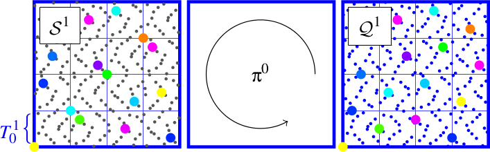

Niveau 2, 2-D, $K=4$
Ensuite, on scramble les points dans chaque tuile $\mathcal{T_1^{i}}$ de $\mathcal{Q_1}$ pour obtenir un spectre globalement bruit bleu.

Et ainsi de suite ...
Garanties
Si l'ensemble initial est dyadique en base $K$ (et donc est basse discrépance), notre ensemble de permutations locales préserve la dyadicité de cet ensemble (et donc la basse discrépance).
Garanties
Si l'ensemble initial est dyadique en base $K$ (et donc est basse discrépance), notre ensemble de permutations locales préserve la dyadicité de cet ensemble (et donc la basse discrépance).
Si l'ensemble initial est dyadique en base $K$ (et donc est basse discrépance), notre permutation globale préserve la dyadicité de cet ensemble (et donc la basse discrépance).
Garanties
Si l'ensemble initial est dyadique en base $K$ (et donc est basse discrépance), notre permutation préserve la dyadicité de l'ensemble (et donc la basse discrépance).
Pipeline final

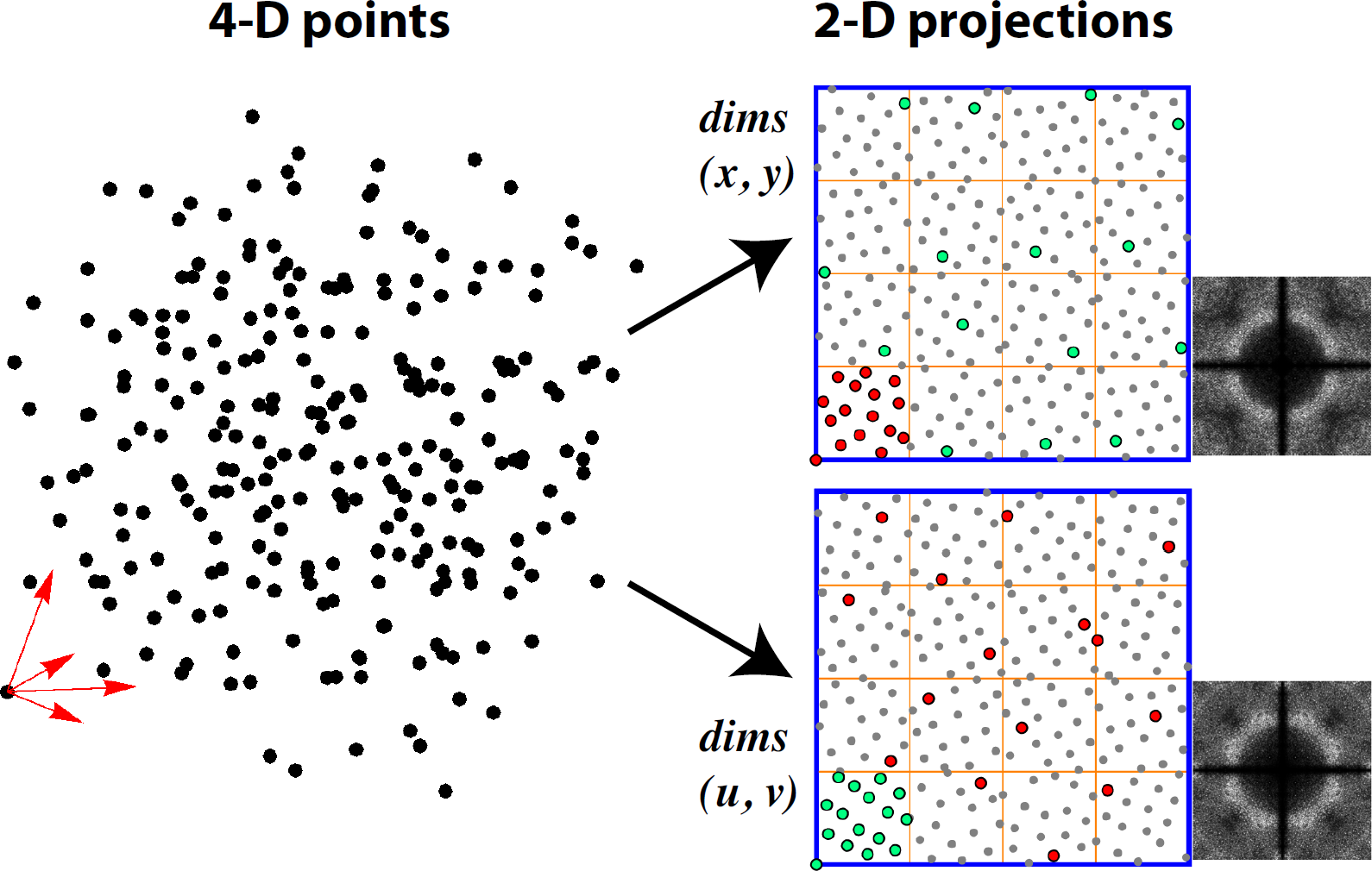
n-D
n-D obtenu par scrambling indépendant de projections 2D.
Adaptative sampling
Results
|
 |
| BNOT [GBO+12] | Owen's Scrambling [Owe95] |
|
 |
| LDBN | MultiProj |
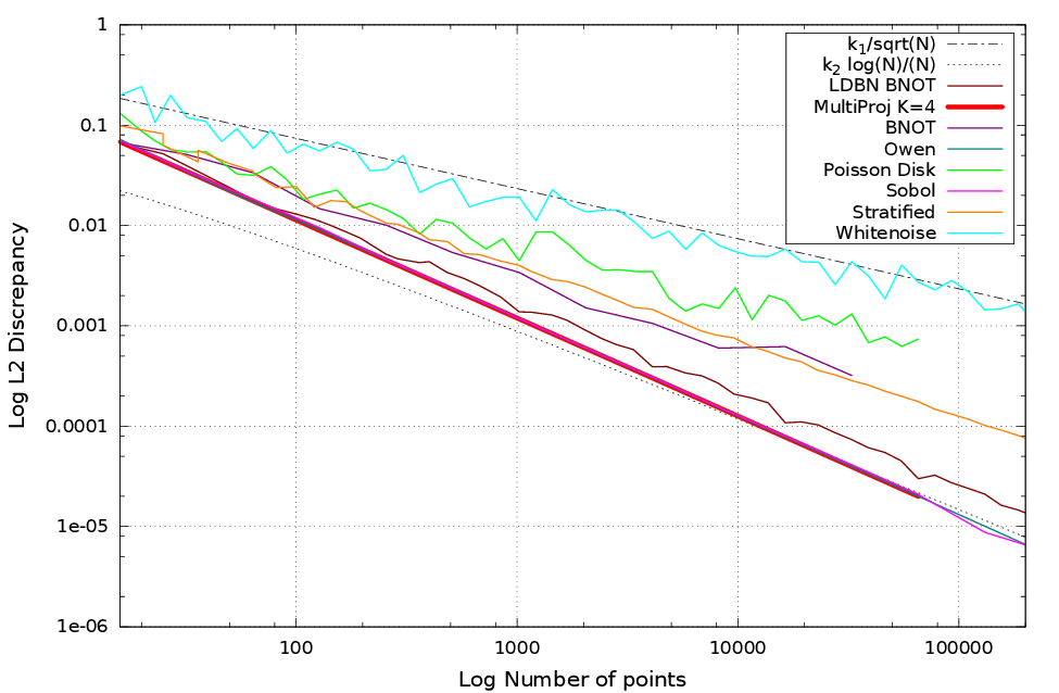
Results
Results
Results

Results
Results
Results
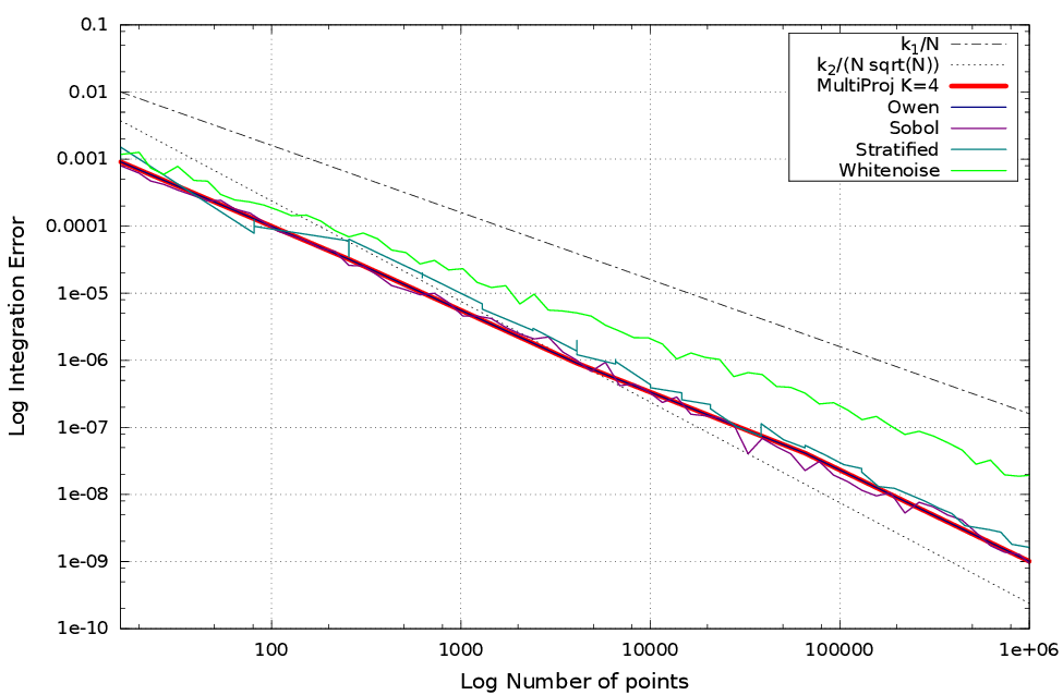
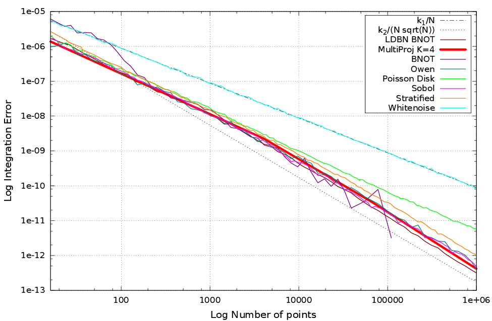
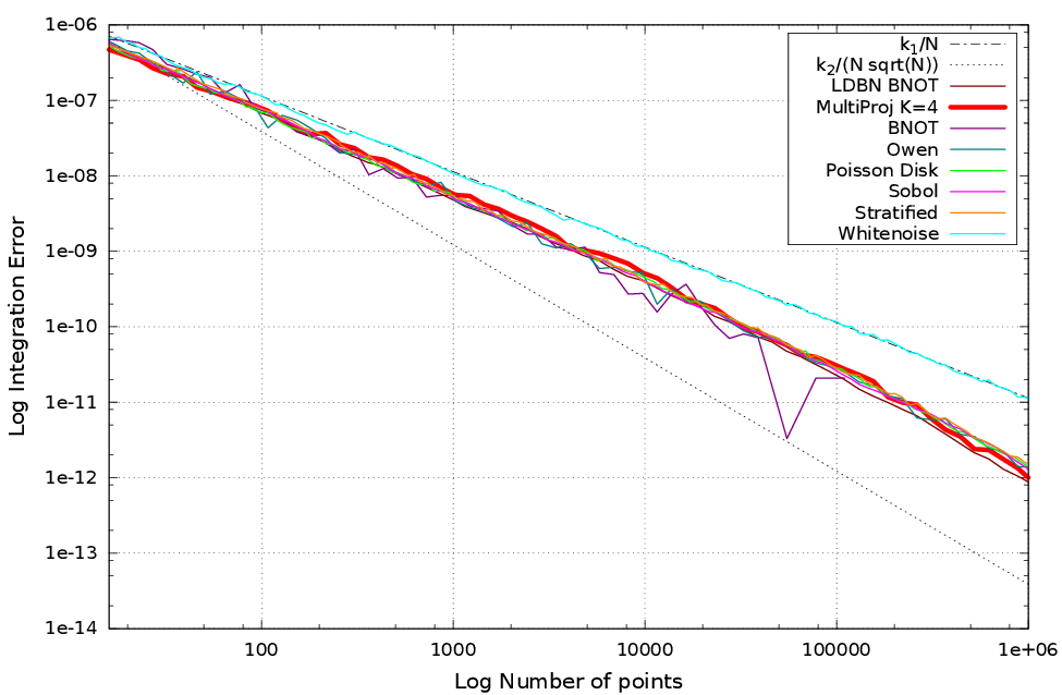
n-D
En fonction de $K$ on peut optimiser un certain nombre de dimensions.
Results


Echantillons 4-D, 16 samples per pixel.
 |
 |
 |
 |
| Stratified (MSE:0.0022) | Sobol [Sob67] (MSE:0.0018) | Owen's Scrambling [Owe95] (MSE:0.0017) | MultiProj K=8 (MSE:0.0018) |
Results

Echantillons 10-D, 16 samples per pixel.
 |
 |
 |
 |
| Stratified (MSE:0.0017) | Sobol [Sob67] (MSE:0.0015) | Owen's Scrambling [Owe95] (MSE:0.0016) | MultiProj K=8 (MSE:0.0013) |
- n-D
- Fast, adaptive
- Blue Noise Discribution for pairs of dimensions
- Sequence
- Low discrepancy in 2D projections only
- Good discrepancy in nD
- Tradeoff between being Low Discrepancy and Spectrum quality
- Still have some permutations to precompute offline
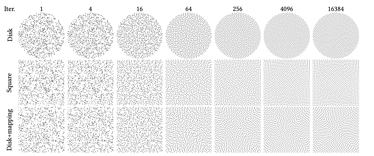
Sliced Optimal Transport Sampling
Advanced topics
Sampling non-uniform densities
General idea
Objective: sample a 2D joint density function $p(x,y)$
Compute marginal density: $$p(x) = \int p(x,y)dy$$ Conditional density function: $$p(y|x)=\frac{p(x,y)}{p(x)}$$ Idea: estimate the marginal in one direction, sample $y$ according to this 1D marginal pdf
Options:
- compute an area-preserving parametrization of $p(x,y)$
- compute the analytical marginals when possible
- estimate them using tabulated approaches
Example: sampling of a triangle
 $\Rightarrow$
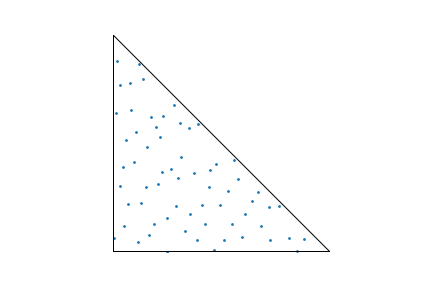
$$ s = (1-\sqrt{u_1}) A + u_2\sqrt{u_1} B + \sqrt{u_1}(1-u_2) C$$
with $u_1$, $u_2$ unform samples in $[0,1)$
Sampling non-square domains
Change of variables + unitary det of the Jacobian $\Rightarrow$ Area0 preserving mapping
Classical domains in rendering
$$x=cos(2\pi u_2)\sqrt{1-u_1^2}\\ y=sin(2\pi u_2)\sqrt{1-u_1^2}\\ z=u_1$$
But also
- Disk
- Cosine-weighted hemisphere
- Cone
- Camera ray
- Piecewise-constant 2D distributions
Metropolis, Markov chain,...
Sample $p(x)$ by just probing the function (no marginal nor
integration)
Sketch of the algorithm:
- Draw sample $x_0$ in $\Omega$
- while I'm done
- Compute the mutation of $x_i$ to construct $x'$
- Evaluate the "acceptance" of $x'$, $a=accept(x_i,x')$
- if $(U(0,1) < a)$ then $x_{i+1} = x' $
- Record $x_{i+1}$
Key ingredients
- Mutation strategy: $T(a\rightarrow b)$ the PDF to mutate $a$ to $b$ (e.g. random walk $b= (a+ \alpha u)$ mod 1, $u\in\mathcal{U}(0,1)$)
- Acceptance strategy: $accept(x,x')= min\left(1,\frac{p(x')T(x'\rightarrow x)}{p(x)T(x\rightarrow x')}\right)$
- + many tricks to avoid start-up bias
- may converge to a sampling of $p(x)$
Bayesian approaches, Markov Chain Monte Carlo, density estimation...
Variance reduction tricks: Importance Sampling
Estimate $\int f(x)dx$ using $$ I_n= \frac{1}{n}\sum \frac{f(s_i)}{p(s_i)}$$ with a distribution $p(x)$ as close as possible to $f(x)$.
(weighting of the sample contributions w.r.t. estimate distribution $p$)
Ideal example: $p(x) := cf(x)$, then $Var(I_n)=0$
Importance sampling may increase the variance but there are many situations / technical ways to estimate $p(x)$ that improve the convergence
Variance reduction tricks: Multiple Importance Sampling
Estimate product of functions $\int f(x)g(x)dx$.
Questions:
- same sampling strategy for both? e.g. $h(x):=f(x)g(x)$
- Different strategies for $f$ and $g$ but how to weight them?
$$ I_n= \frac{1}{n_f}\sum_{n_f} \frac{f(s_i)g(s_i)w_f(s_i)}{p_f(s_i)} + \frac{1}{n_g}\sum_{n_g} \frac{f(s'_i)g(s'_i)w_g(s'_i)}{p_g(s'_i)}$$
For instance using the balance heuristic: $$ w_\bullet(x) := \frac{n_\bullet p_\bullet(x)}{\sum_i n_ip_i(x)} $$
or the power heuristic: $$ w_\bullet(x) := \frac{(n_\bullet p_\bullet(x))^\beta}{\sum_i (n_ip_i(x))\beta} $$

Variance reduction tricks: Control Variate
Instead of estimating $I=\int_\Omega f(x)dx$ using M.C., we
estimate
$$ I= \int_\Omega f(x) -\alpha h(x)dx + \alpha H$$
where $h(x)$ is the control variate
(and
$H=\int_\Omega h(x)dx$ and $\alpha$ the strength of the control)
Then,
$\langle I^*_n\rangle=\langle I_n - \alpha H\rangle + \alpha H$
choosing an optimal coefficient $\alpha=Cov(\langle I_n\rangle,\langle H_n\rangle) /
Var(H_n)$,
we have
$$Var( I^*_n) = Var( I_n) (1 -
Corr(\langle I_n\rangle,\langle H_n\rangle)^2)$$
Example:
- $ I=\int_0^1 f(x)dx$, with $f(x)=\frac{1}{1+x}$
- $ I_n= \frac{1}{n}\sum f(s_i)$,
- sample $g(x)=1+x$ with $\int_0^1 g(x)dx=\frac{3}{2}$
- $I_n = \frac{1}{n} \sum f(s_i) + c g(s_i) - c\frac{3}{2}$
$n=1500$, variance reduction from 0.01947 to 0.0006