Computational Geometry: Digital Delaunay Triangulation and Applications§
| author: | David Coeurjolly |
|---|
| author: | David Coeurjolly |
|---|
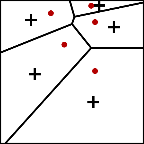
Input
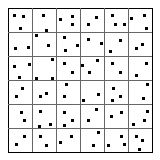
local consistency of points
![[0,N]^d](_images/math/3950b2b1cd998a687b8fad7f54f86ca1536694f9.png)
specific integer based structures
Let’s start with good news
… and the bad ones
 perturbation can be done
Questions
Can we expect better bounds for Delaunay structure?
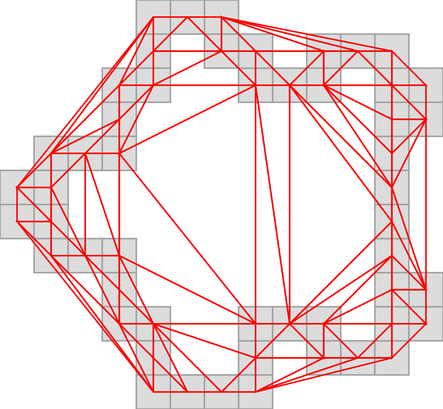
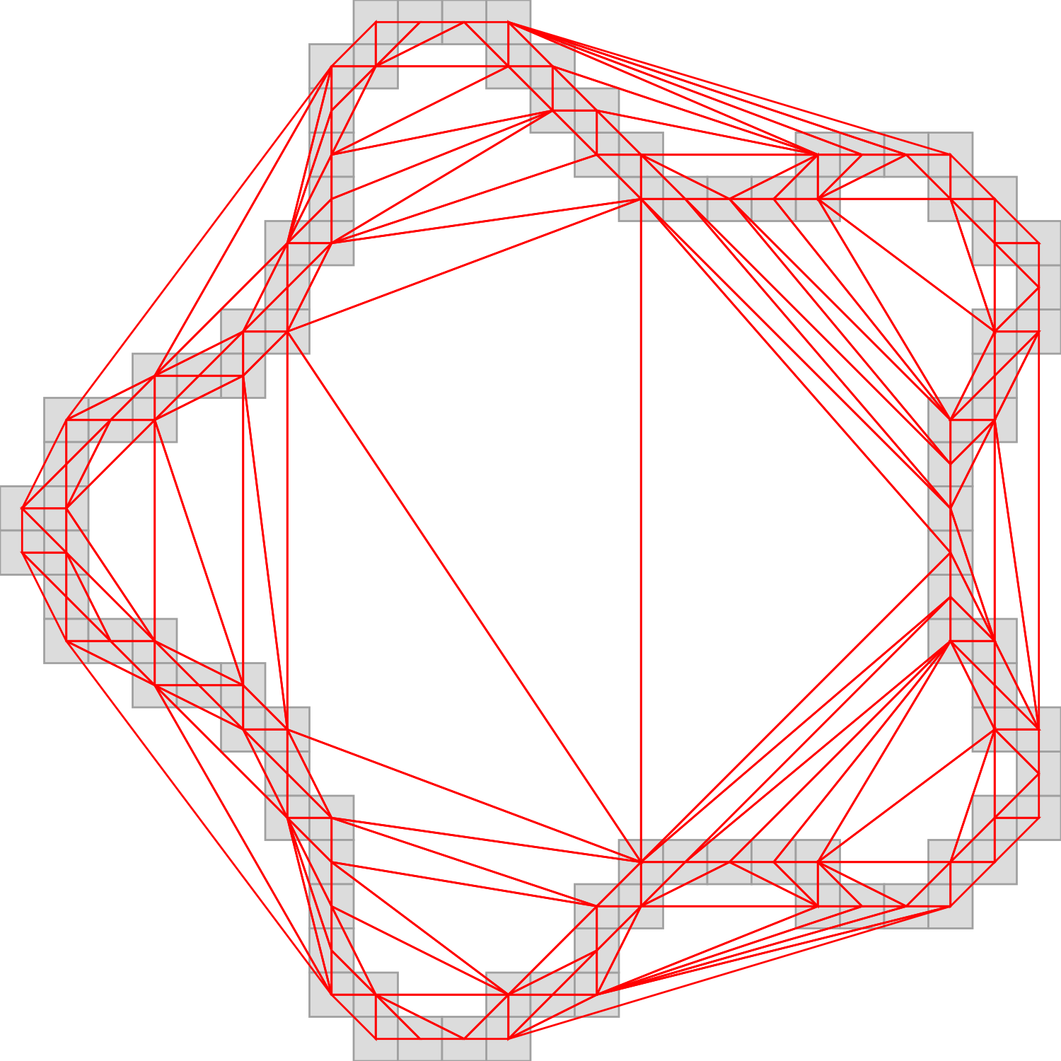
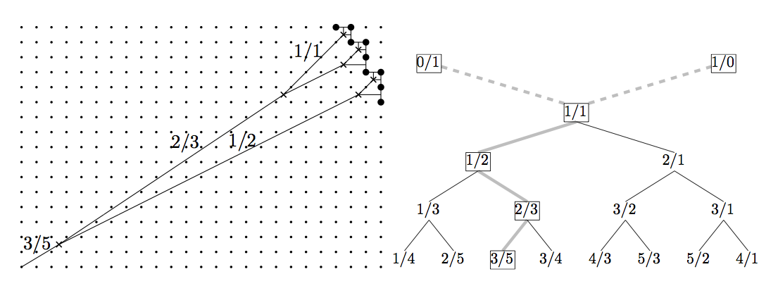
Delaunay triangulation from minimum spanning tree
Thm. [Devillers]
If the Euclidean Minimum Spanning Tree of the input point set,
the whole triangulation can be constructed in expected time 
( hence for
  ,
,  ,
,  for
for  )
)
Why?
Main observation
Thm.
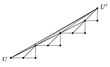
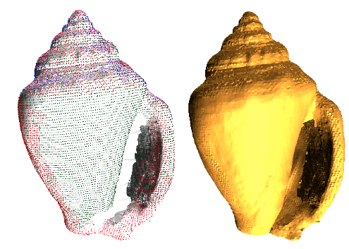
The polyline defined from digital contour points is a Delaunay spanning graph with maximal degree 2
Thm.
Expected time for Delaunay construction for digital contour is in 
|
|
|
Observation
For digital straight segment patterns, can we recover the Delaunay structure from arthimetic properties?
 Yes! [Roussillon, Lachaud]
Setting
 domain
Main Result
Thm. [Chan]
 expected randomized time for Delaunay Triangulation construction
Key Data Structure: Van Emde Boas Tree
 !!
!!Settings
Set  with
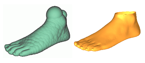
with  points sampling/approximating a smooth 2-manifold C can I reconstruct a discrete manifold M such that
 for some metric d (e.g. Haussdorff)
Variants
has good sampling properties (e.g. at least
  ), then for samplings with
 Algorithm A produces a discrete structure
homeomorphic to C
Algorithm A produces a discrete structure
homeomorphic to CSampling Definition
Def.
is an -sampling of  if
if
 and
and  ,
,  such that
  .
.
with lfs(x) being the local feature size at x: 
-samples are on is be used to control the number of samples and its
distribution.Question what does  mean?
mean?
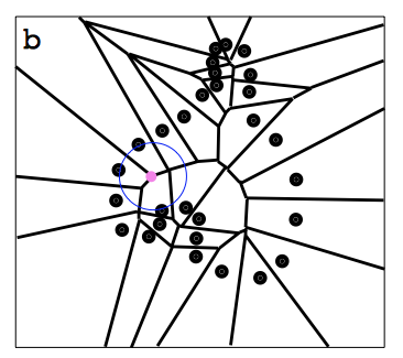
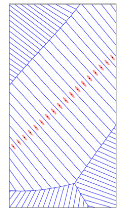
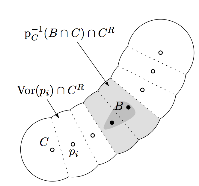
| Compute the Voronoi Diagram of |
|
| Compute the Voronoi Diagram of |
|
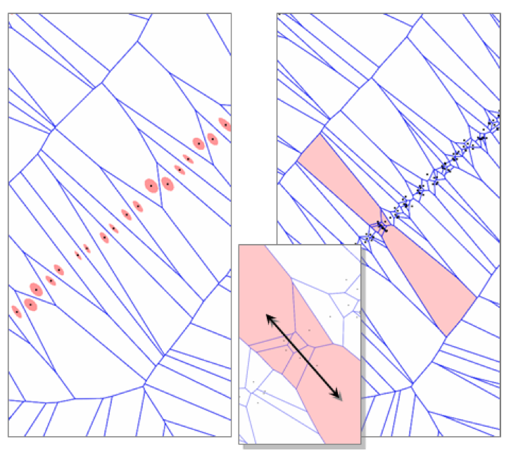
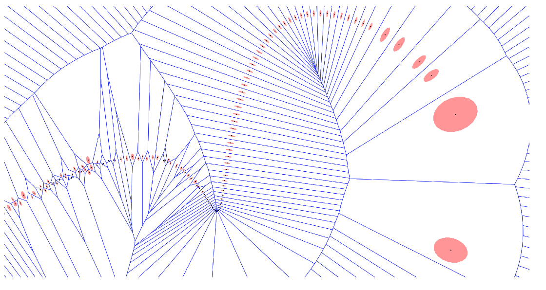
| Extract the poles and polar balls | 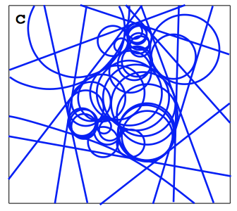
|
pole of a sample s: pair of power diagram vertices farthest from s on either the inside or outside of the “object”.
| Compute the Voronoi Diagram of |
|
| Extract the poles and polar balls |
|
| Compute the Power Diagram of such poles | 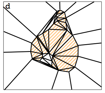
|
| Compute the Voronoi Diagram of |
|
| Extract the poles and construct |
|
| Compute the Power Diagram of such poles |
|
| Extract the power crust | 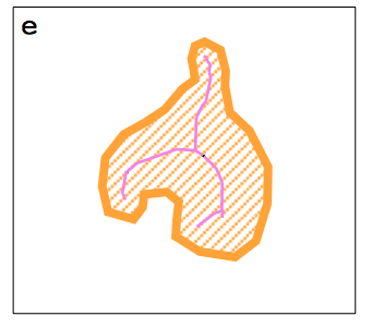
|
Thm.


|
|
Side-product of Power Crust
Thm.
Direction  from poles
  and
and
 at a sample s is a convergent
(w.r.t. ) estimation of the normal
direction at s
at a sample s is a convergent
(w.r.t. ) estimation of the normal
direction at s
…but very sensitive to noise or sampling conditions
keep in mind that in theorems, samples C exactly
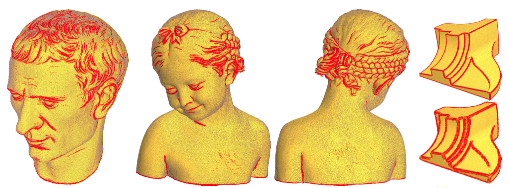
Alternative solutions: use Voronoi cell covariance matrix [Alliez]
Idea
Covariance matrix is still a key tool but it is evaluated on r-offest of the input set
Thm.
Eigenvalues/Eigenvectors of the covariance matrix at a point are related to principal curvature/principal curvature direction
Convergence results exist with Haussdorff hypothesis on the point set
Robust tool for feature extraction
Idea
Estimate
from
 |
|
Many fields
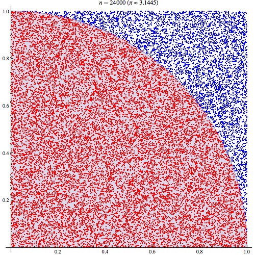
Variance in the Monte-Carlo Integration process (uniform sampling)

Integration error :
Spectral properties
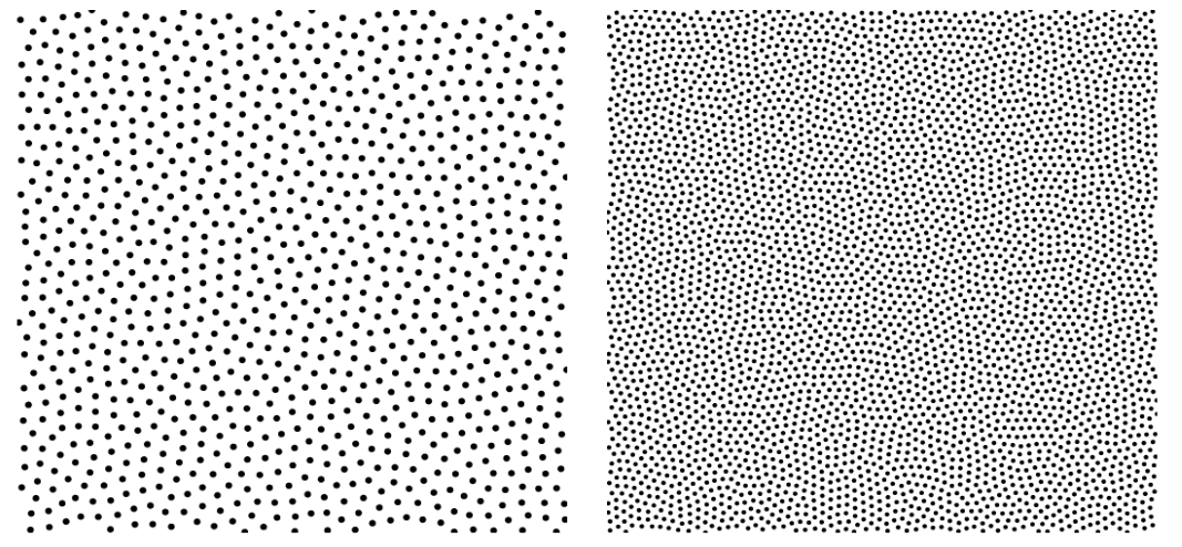
Uniform sampling
Jittered/Stratified sampling
Poisson Disk
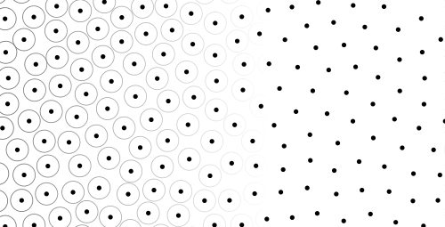
Low discrepancy sequences Quasi-Monte-Carlo approaches
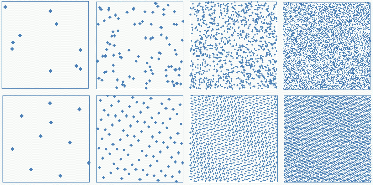
Tiled based approaches
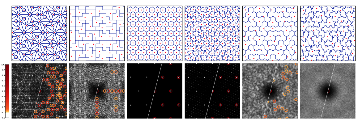
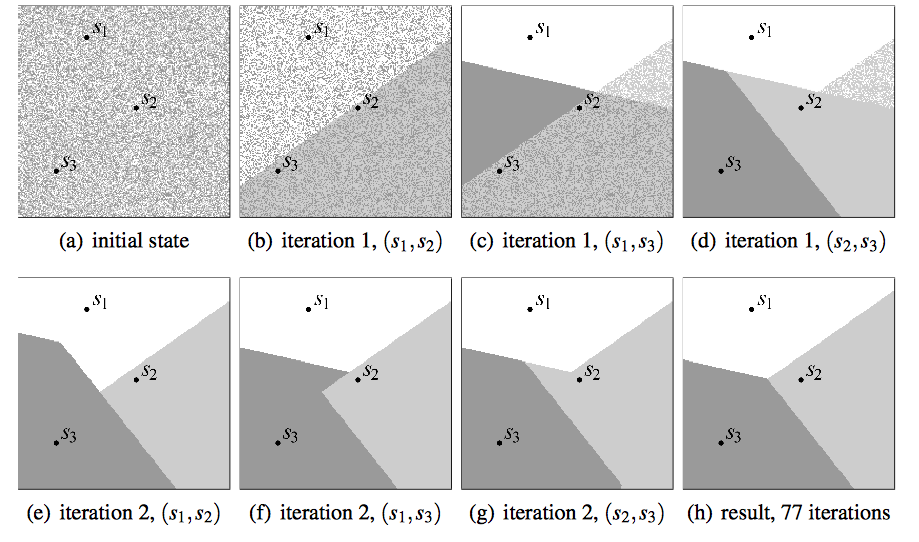
Description Iterative algorithm
Generate N points using uniform sampling
Compute its Voronoi diagram V

while (not(stability))
{
   For each cell
     Compute its centroid
     Move site to the centroid
}
|
|
|
|
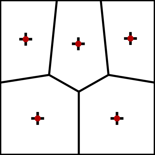
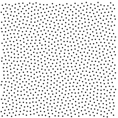
Converges to a stable structure (honeycomb) but if we stop the process, we obtain a reasonable point sampling
[Cohen-Steiner et al]
Equi-distribution of samples  Cells with same capacity
Isotropic influence zone of samples Energy model on
cell shapes
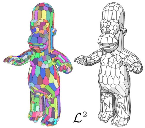
iterative process to minimize global energy related to power diagramDiscrete version
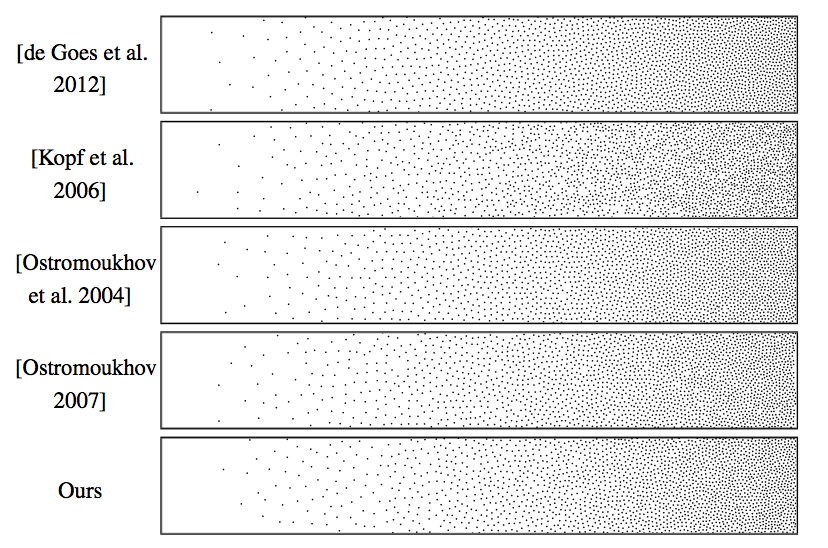
Experimental comparison
|
|