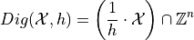
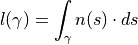
Digital Geometry: Estimators§
| author: | David Coeurjolly |
|---|
| author: | David Coeurjolly |
|---|
Objectives
e.g.
Algorithmic point of view
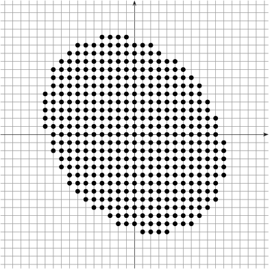
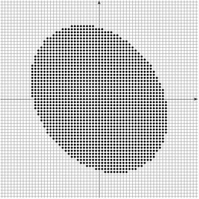
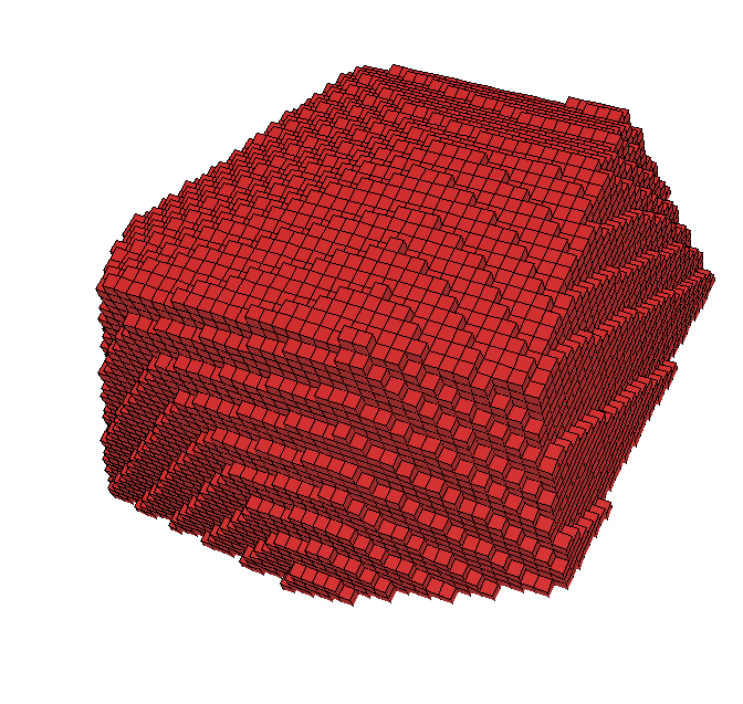
Multigrid analysis Gauss digitization scheme parametrized by a grid-step
|
|
|
Idea
Single scalar quantity attached to a digital object 
E.g.:
Area in 2D (resp. 3D)
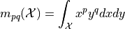
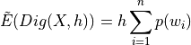
Geometrical moments:
Multigrid convergence definition
Def.
 of some geometric quantity
  is multigrid convergent for a family of shapes
  and a digitization process
  iff for all shape
  , there exists a grid step
  such that the estimate
  is defined for all
  and
and
where  with null limit at
  . This function is the speed of convergence of the estimator.
From previous lectures…
 , this estimator converges for convex shapes with speed
  [Gauss, Dirichlet], this estimator converges for
  convex shapes with speed
  [Huxley]
| Quantity | 1 | 0.1 | 0.01 | 0.001 | … |
|---|---|---|---|---|---|
| h | 1 | 0.1 | 0.01 | 0.001 | … |
 |
1 | 0.04328 | 0.00187 | 0.00008 | … |
Idea
We specify:
A set of elementary displacement or pattern (e.g.  and
and  )
)
A weight per displacement vector
Length Estimation sum of weighed occurrences of each pattern
 statistical analysis to optimize the weights to minimize errors for random distribution of segments of length

Generalizarion
We decompose the  into pattern of length
For each pattern  , we consider a weight
Main Result
Thm.
 and
and  the set of slopes
  such that the estimator is convergent is countable most of the time, the estimator does not converge
[Tajine,Daurat]
Solution locally adapt the parameter m ? set m as a function of h ? ( )
)
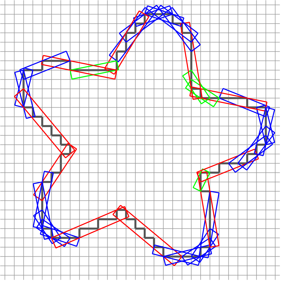
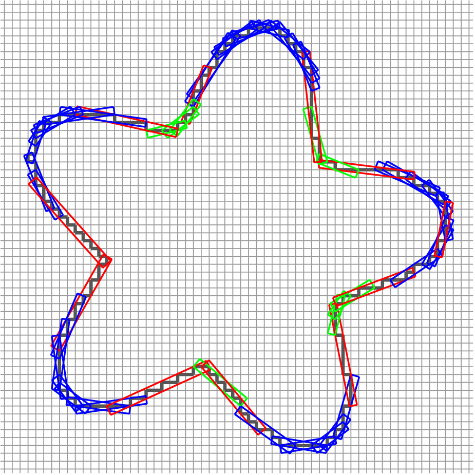
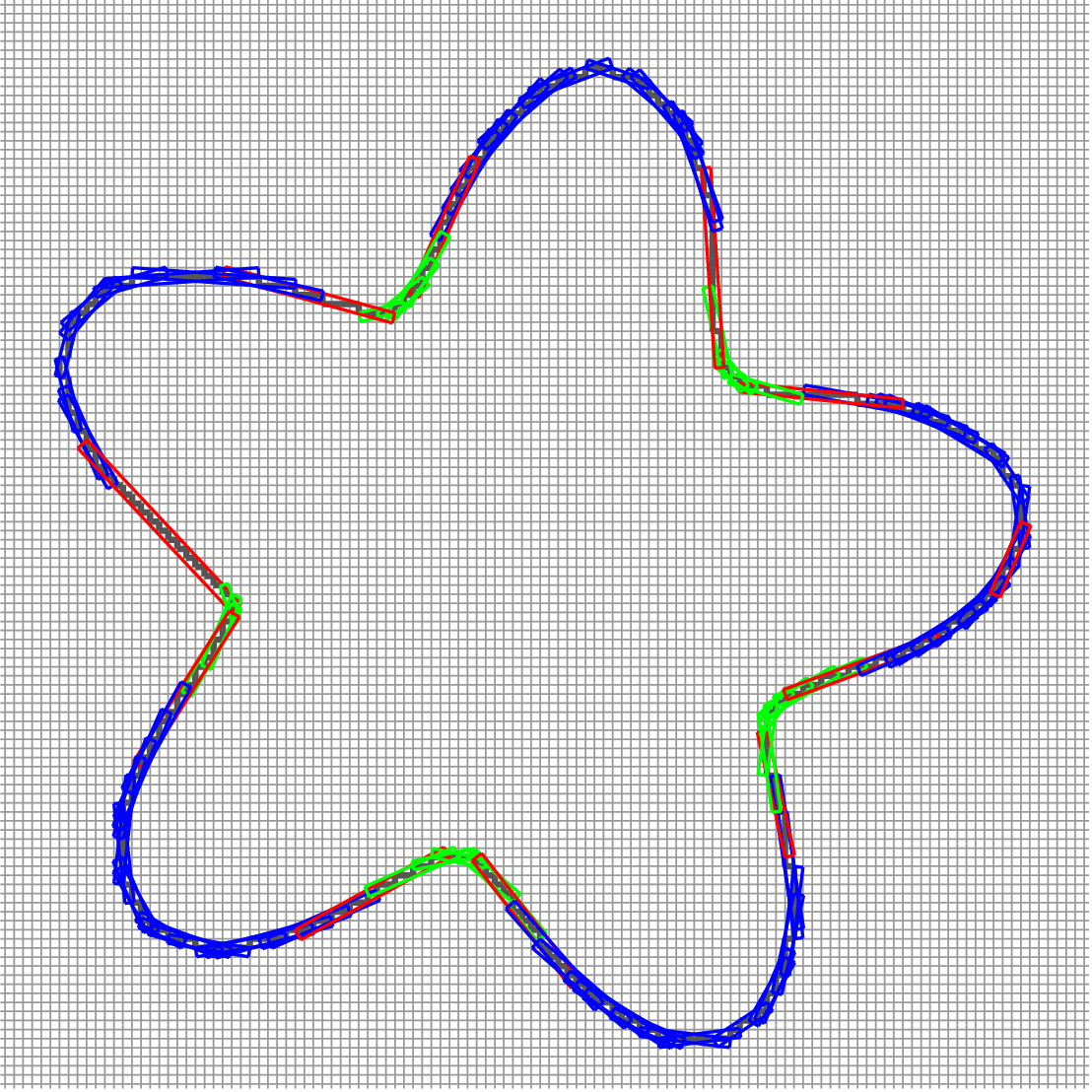
Basic Idea
Compute the decompostion of the contour into maximal DSS  (with thus
 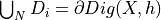 )
)
Main result
Thm.
 is multigrid convergent for convex shapes with speed
We need
is defined
|
|

|
|

|
|

|
|

|

|
|
|
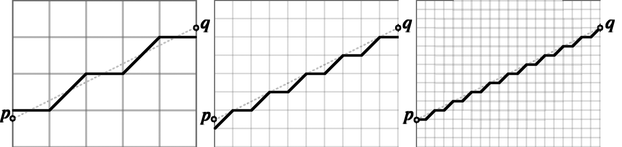
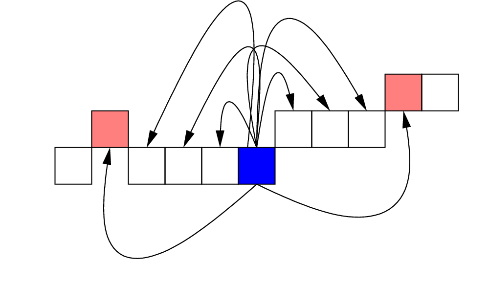
Principle
 defines a piece of the contour from index
  to
to 
 (e.g. being a DSS, a DCA,…)


 is maximal if
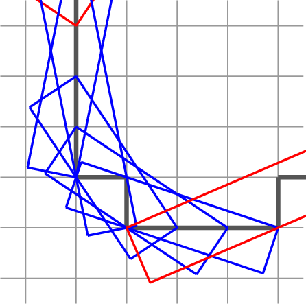
Maximal covering = set of all maximal segment of
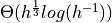
Algorithmic point of view
 per operations


|
|
|
|
|
|
|
|
|
| X |  |
 |
 |
Useful to
Idea digital version of
Hence:
Main result: If  uniformly converges in
  ,
,  converges in
Multigrid convergence for local geometric quantities
Def.
The estimator  is multigrid-convergent for the family if and only if, for any , there exists a grid step such that the estimate
  is defined for all
  with , and for any
  ,
,
with
where  has null limit at 0. This function defines the speed of convergence of toward
  at point x of
  . The convergence is uniform for
  when every
  is bounded from above by a function
  independent of
  with null limit at 0
we need a mapping 
Uniform convergence is a strong constraint
Generic fitting approach
Fix a neighborhood around a point 
Fit the  digital points
  by a function
  with parameter vector
Least-square fitting : Minimize quadratic error:
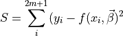
E.g., 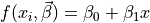 for linear fitting.
Example: tangent vector estimator
 where
where  is the result of a least-square linear fitting
 No convergence results for fixed
Trivial idea Use a kind of symmetric maximal DSS to estimate the tangent
Algorithmic
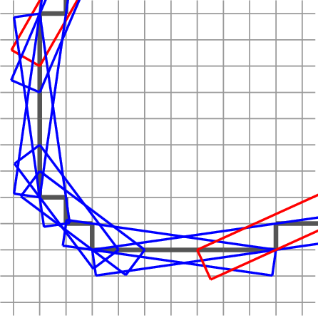
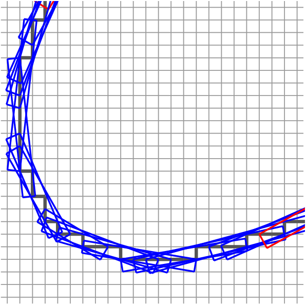
More flexible approach Maximal segment from mxaimal covering
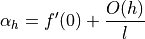
Given a maximal DSS with slopde ![\alpha_h\in[0,1]](_images/math/ade706f8278291ac76337b8f233760f4ad63c121.png) containing point
containing point 
We consider a local parametrization of 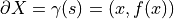
Suppose P=(0,0), we have, ![\forall x\in[0,l]](_images/math/9a1609768269fa4da0485ba4fa9e73853c2f8578.png)

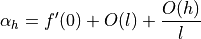
If the curve is locally linear,  , and
, and
If the curve has curvature greater than  , Taylor decomposition gives us:
Convergence Result
Prop.

with 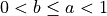
Length of maximal DSS is crucial !
Fitting an order-2 polyonmial
valueChord length approach
 with
with 
 (see below)
Circumscribing circle from two half-tangent
 (see below)
Nice but  is not in
We need to consider the following quantities
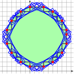
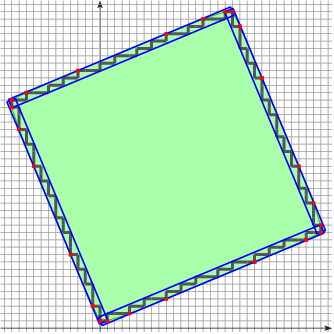
 the number of edges of the convex hull of
  the number of maximal segments in the covering of
  length of convex hull edge
  (
( metric for (1)-contours)
 length of a maximal segment ( metric for (1)-contours)
Then, we want to compute:
valueEverything as functions of h and considering specific shape family
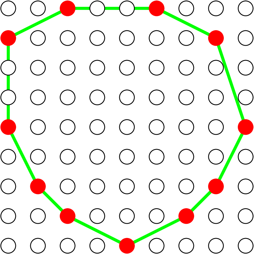
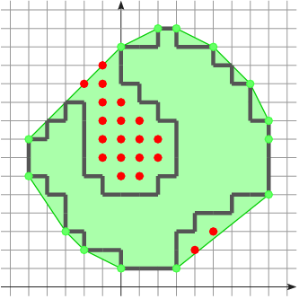
Convex hull of X smallest convex set containing point set X. As consequence of the Def, the convex hull is polygonal convex set with vertices in X
Main result in Lattice polytope in 2D [Barany, Zunic, Balog, Acketa,…]
Thm.
(Similar results in n-D exist)
|
|
|
Main result [Lachaud, de Vieilleville, Feschet]
If  is convex and
|
|
 |
 |
(Length = distance for (1)-contours)
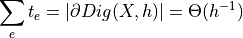
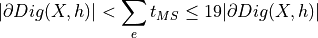
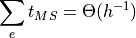
Results on the sum of lengths
From [Lachaud, de Vieilleville, Feschet]
Hence
If is convex and
| Quantity | Smallest MS length | Average MS length | Largest MS length |
|---|---|---|---|
 |
 |
 |
 |
 |
 |
 |
 |
(Hints for  , the lower bound = lower bound on
  / upper bound , results for smallest/largest MS require couple of more steps)
Any slope of MS containing P provides multigrid convergent estimation of tangent at P
Tangent Estimation in 2D
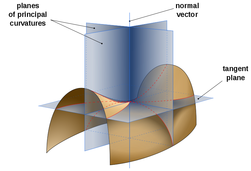
Curvature Estmiation in 2D
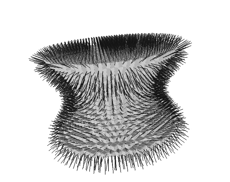
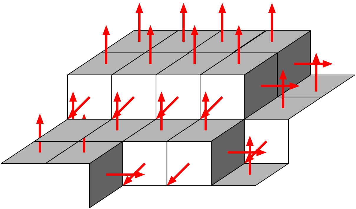
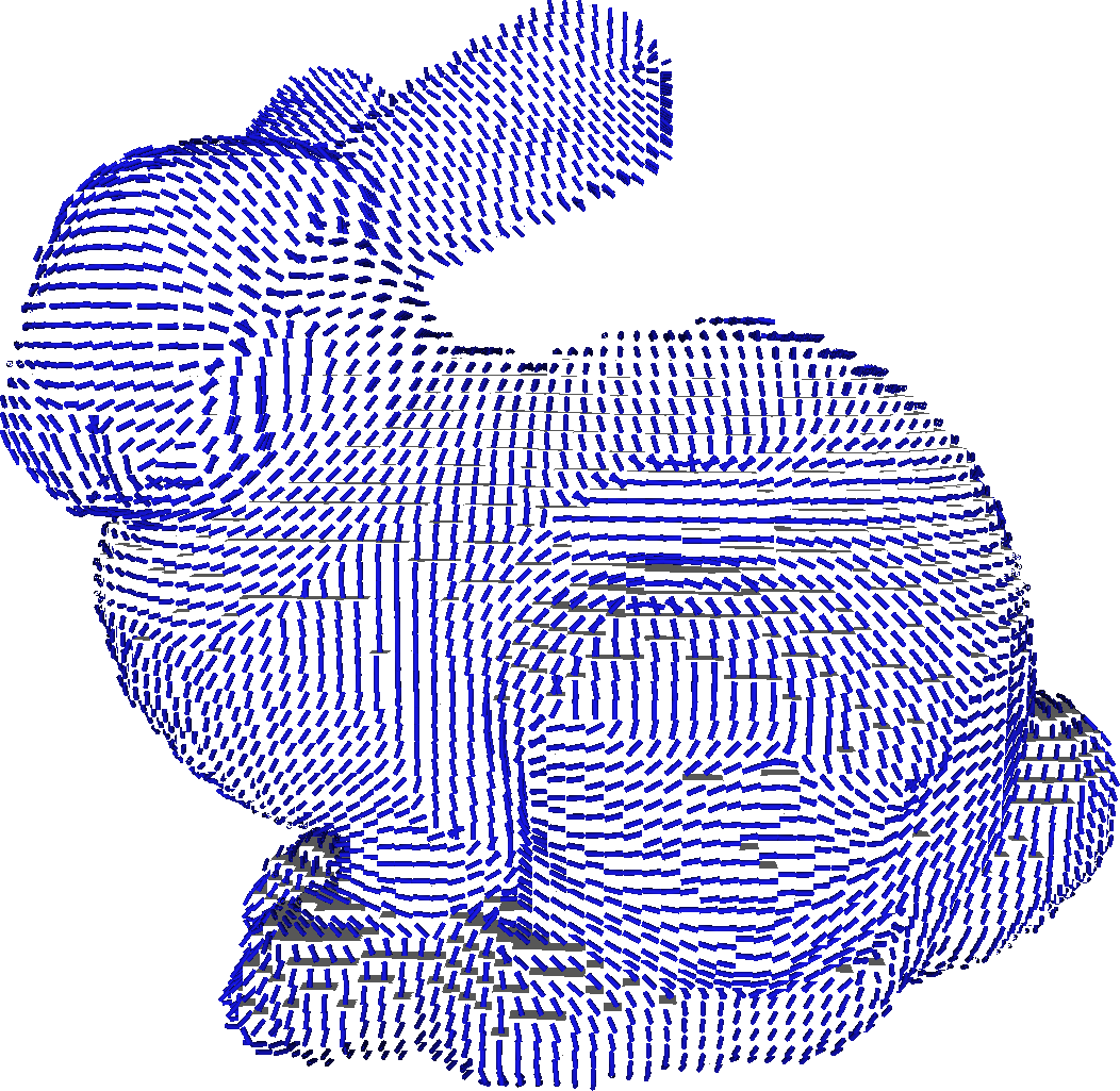
Slice based approaches
normal vectors
|
|
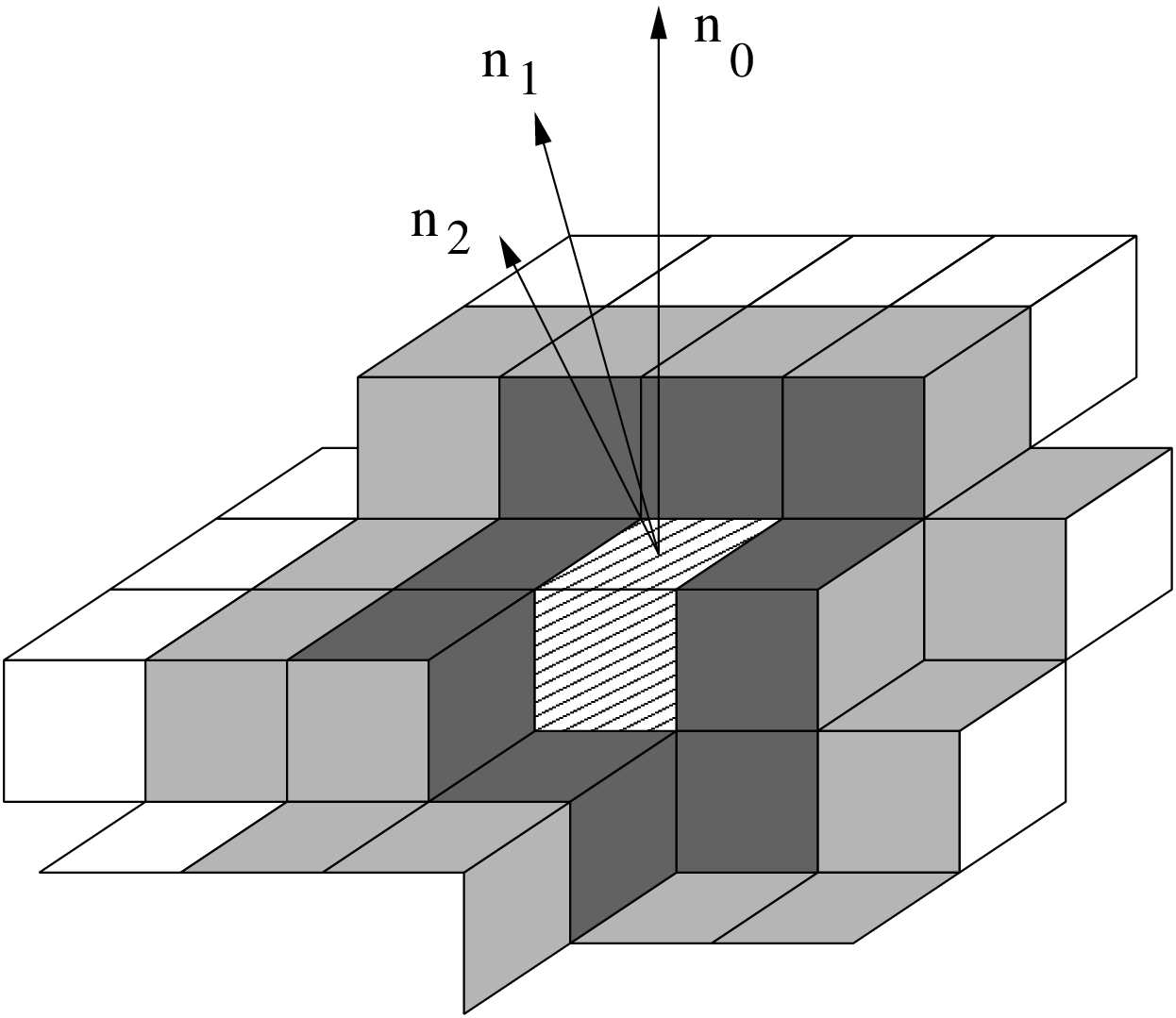
Convolution based approaches
Convolution of elementary normal vectors in a given neighborhood
|
|
still have to fix a neighborhood parameter
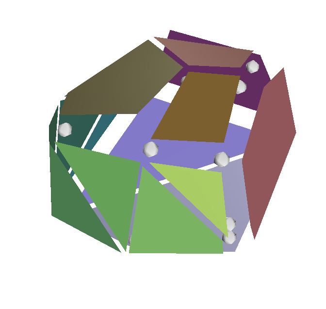
Digital Plane Recognition approaches
… but …
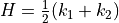
Mean and Gaussian curvature

Fitting an implicit polynomial surface is still doable but we need information on the neighborhood
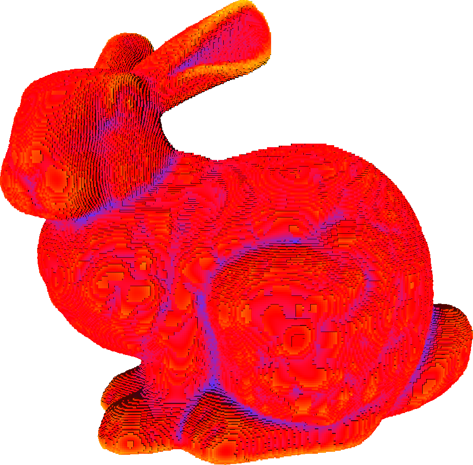
Integral Invariant approach neighborhood in  seems to be required
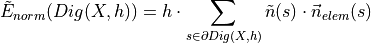
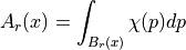
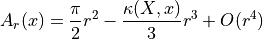
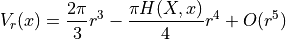
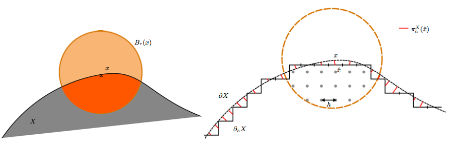
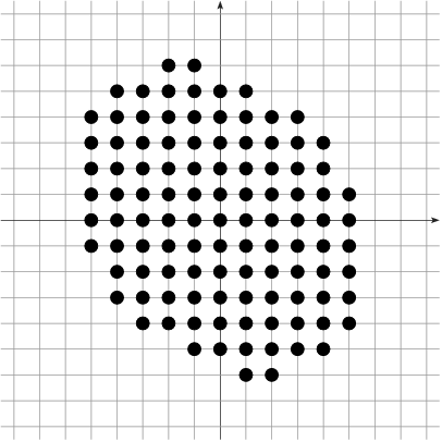
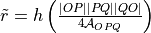
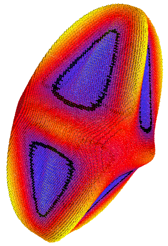
Idea compute area of the intersection between a ball  and at
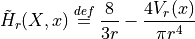
Then, from Taylor expansion and for 
Hence,
 by definition when
 first error term induced by [Gauss,Huxley] (O(h))
 and
and  (back-projection used here)
Main Result
Thm.
For a family of shape with onvex -boundary and bounded curvature,  , for any
  , setting
  , we have


(similar bound in 3D)
Idea
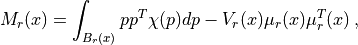
Instead of computing the volume of  , we compute its covariance matrix
Eigenvalues of  are such that:
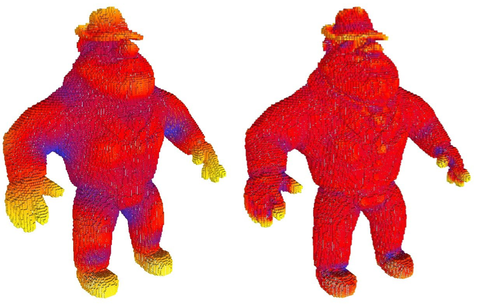
Result
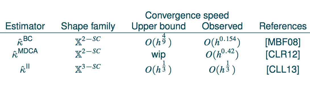
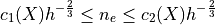
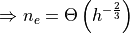
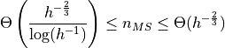
Similar convergence results exist with speed
Experimental analysis confirms the  neighborhood size
|
|
|
|

|
|
First, let’s have a look to the theorem statement
Thm.
For a family of shape with convex -boundary and bounded
curvature, , for any  , setting , we have
…………
, setting , we have
…………
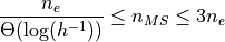
To have the convergence, we need the radius to be in

We know that
Let’s use (square of) average MS length to define r
Parameter-free convergence in
 !
!
Automatic selection of the scale parameter
|
|
|
|
|
|
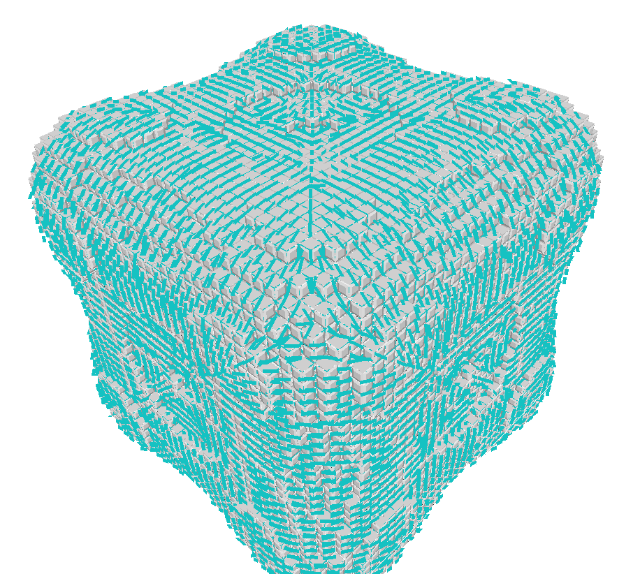
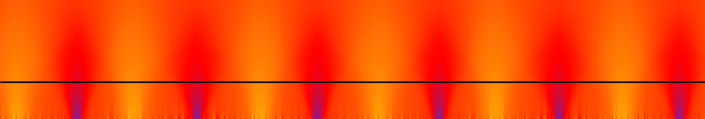
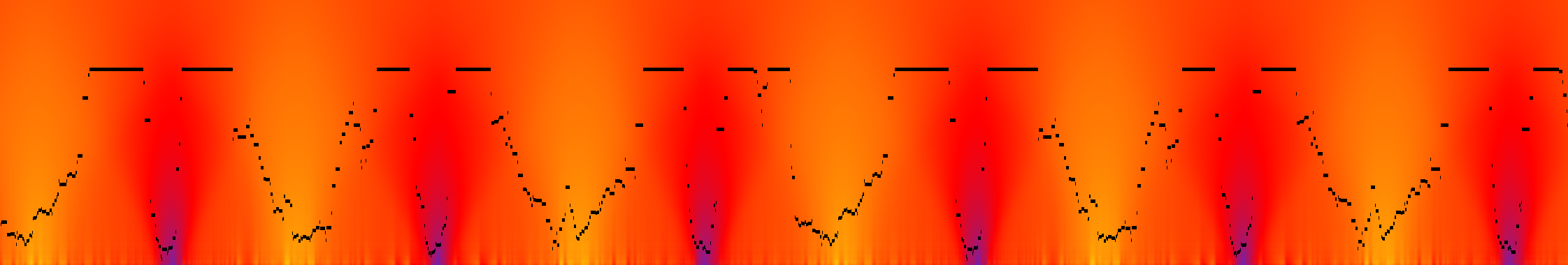
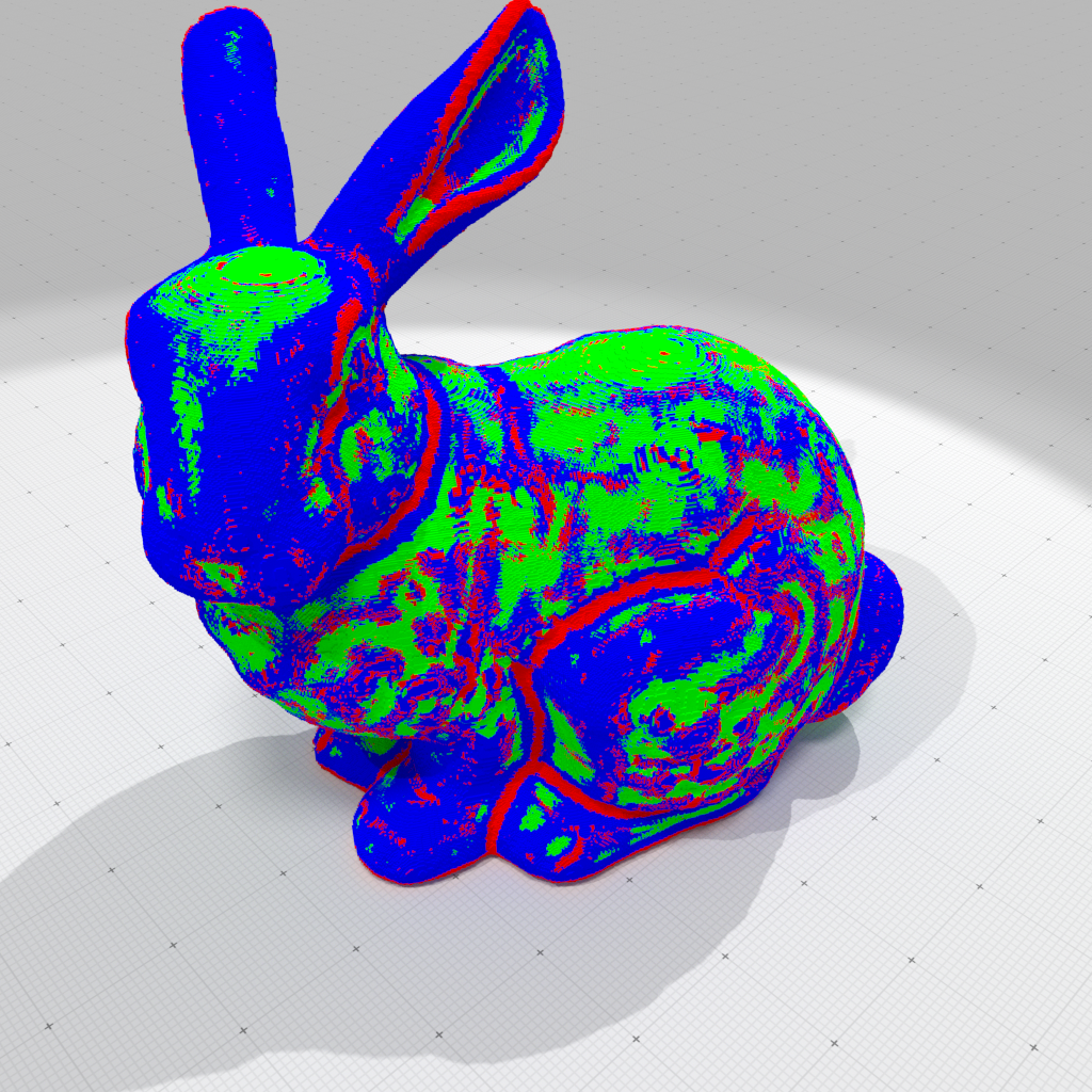
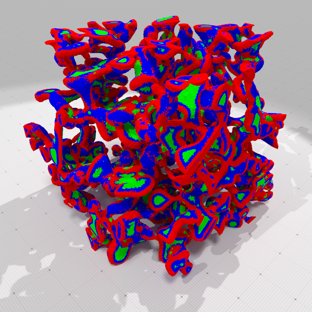
Idea Use scale-space behavior of II estimators to classify surfels into flat,smooth,edge regions
|
|
|
|
Simple definition
 is digitally convex iff there exists
convex shape
is digitally convex iff there exists
convex shape  such that

|
|
Let  be a (1)-curve
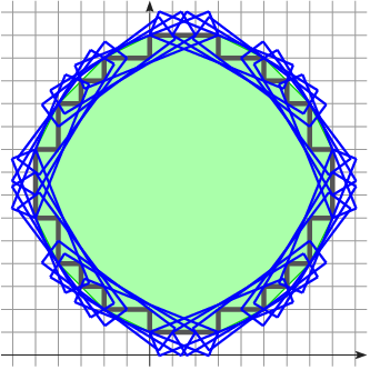
Properties on convex hull
 is a period of some DSS is a leaning point for some period of some DSS
Main result [Debled-Rennesson, Doerksen-Reiter]
Thm.
S is digitally convex  slopes of maximal segment in the covering are monotonic
|
|