Digital Geometry: Contour Analysis§
| author: | David Coeurjolly |
|---|
| author: | David Coeurjolly |
|---|
Objectives
Idea
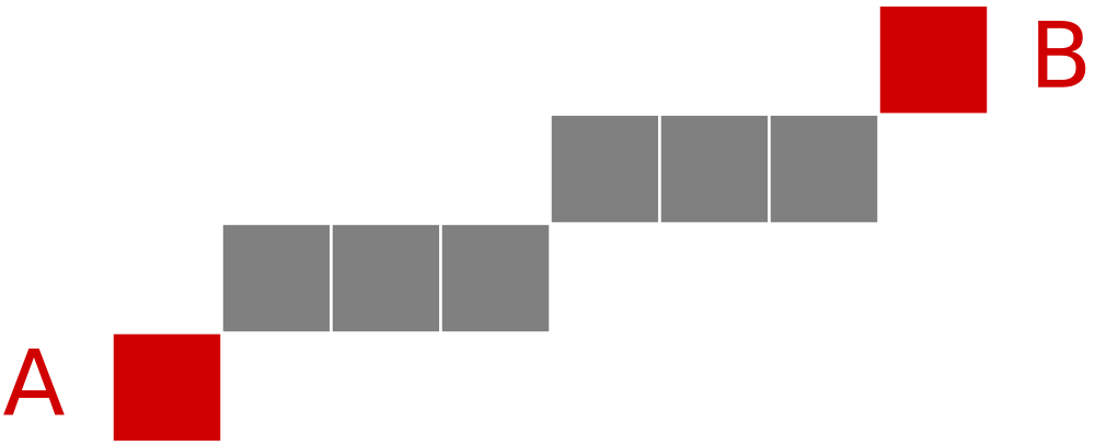
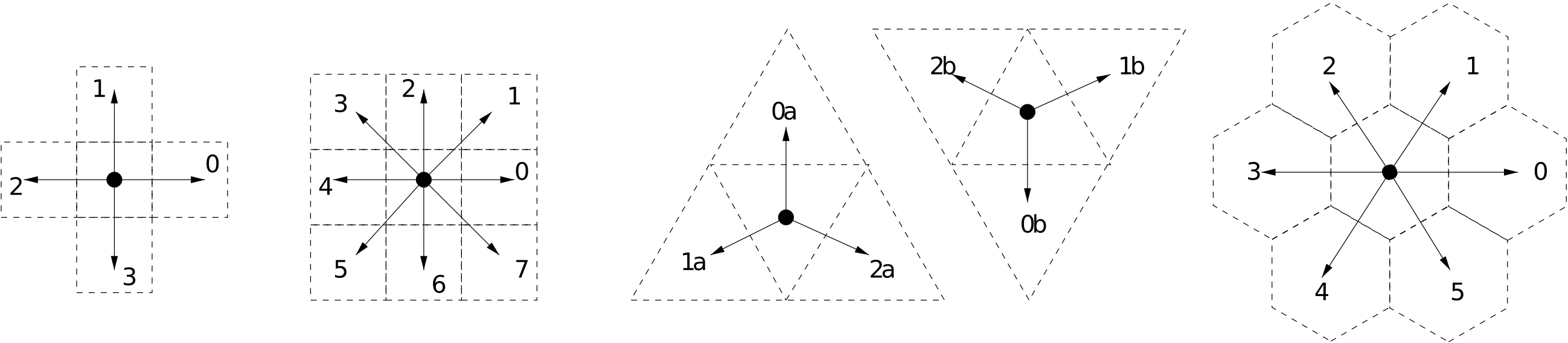
Starting point + differential code according to adjacency displacement and an orientation
Reversible and unique encoding
Code driven geometrical transformations


 (for (0)-adjacency)
Basic length estimator
 for even codes
 for odd codes
Given a (1)-adjacency, let  be the number of ith-code
(but may be self-intersecting)
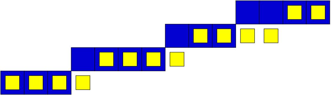
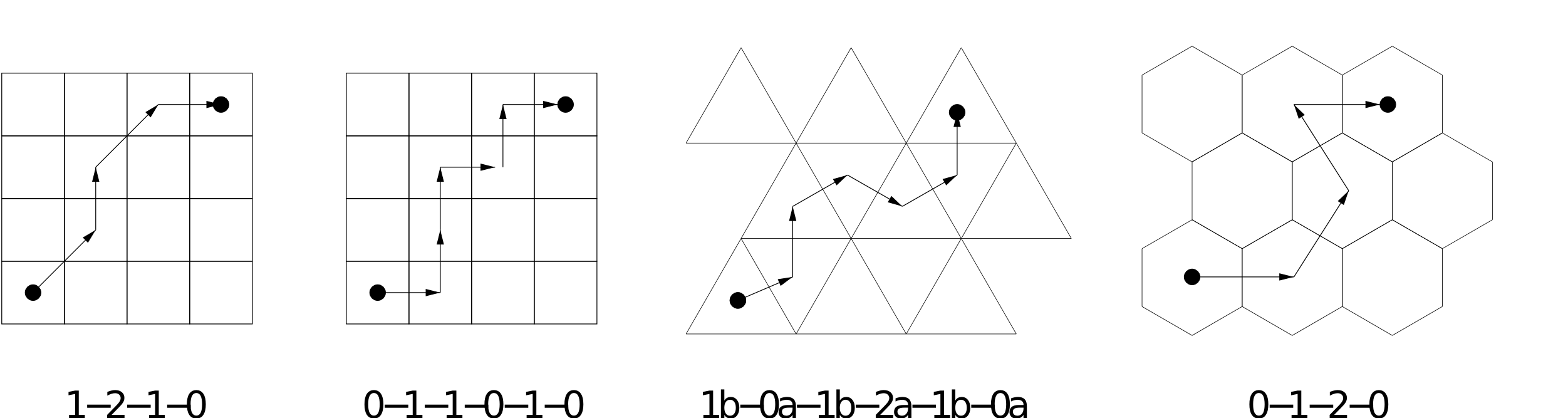
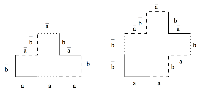
Representation as a word on an alphabet
 …
…
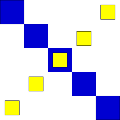
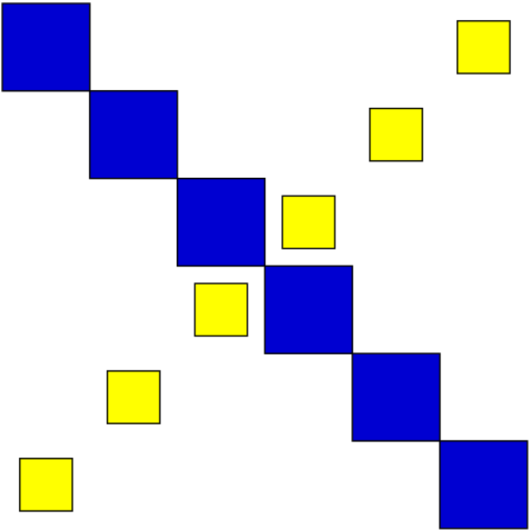
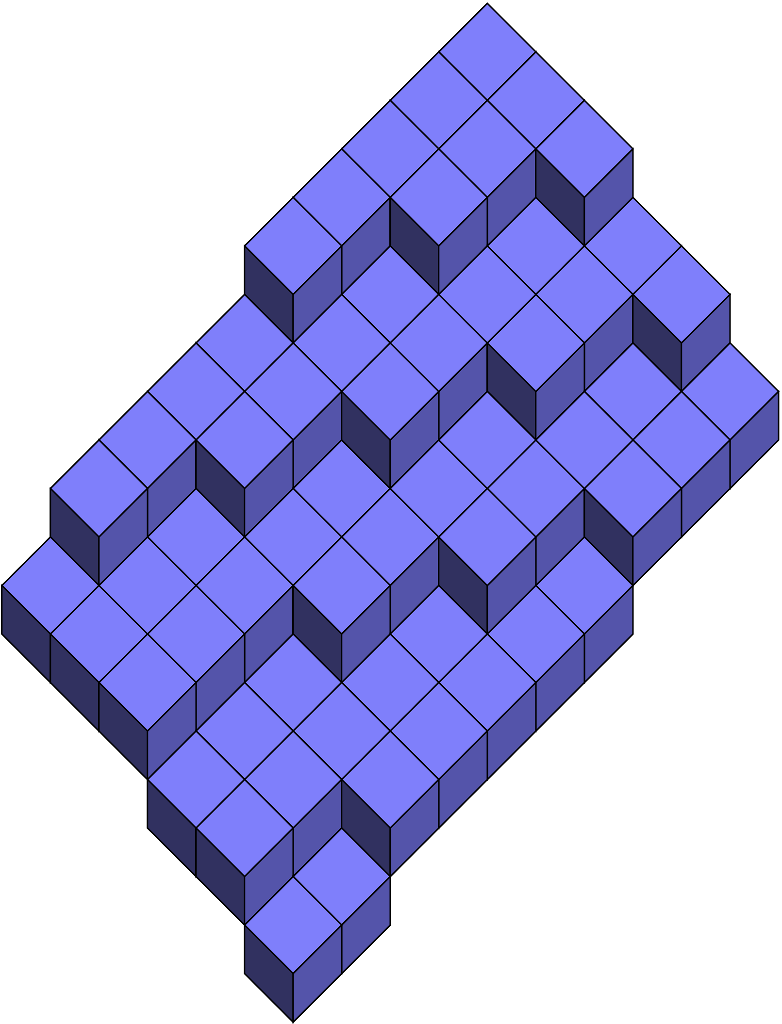
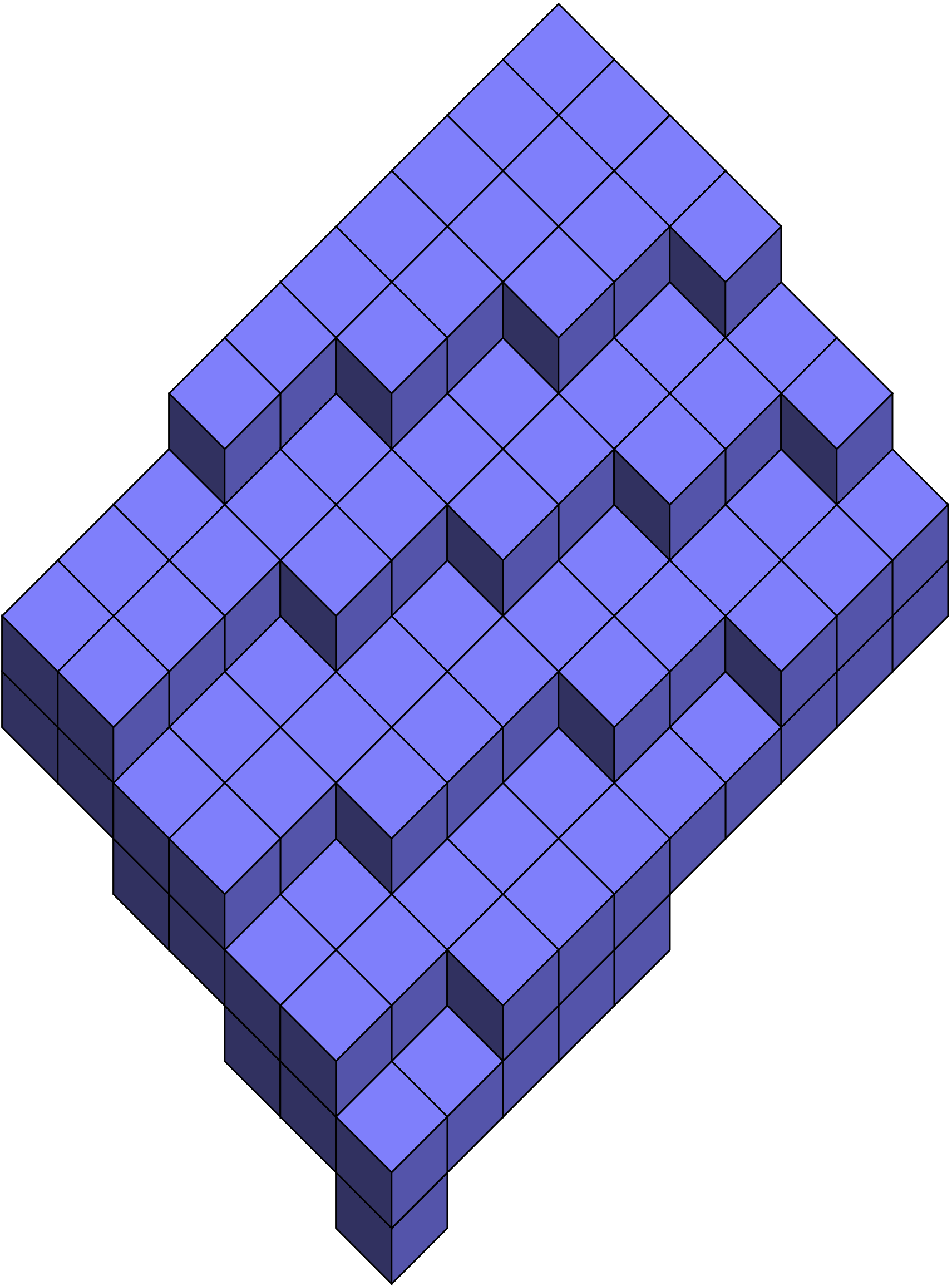
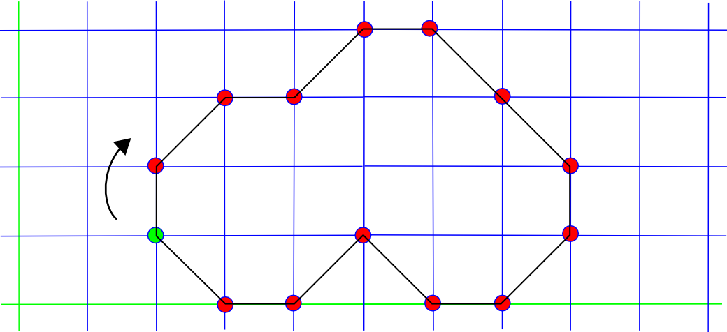
A Polyomino  tiles the plane if and only if its contours has the following structure (up to cyclic rotations)
  [Beauquier-Nivat]
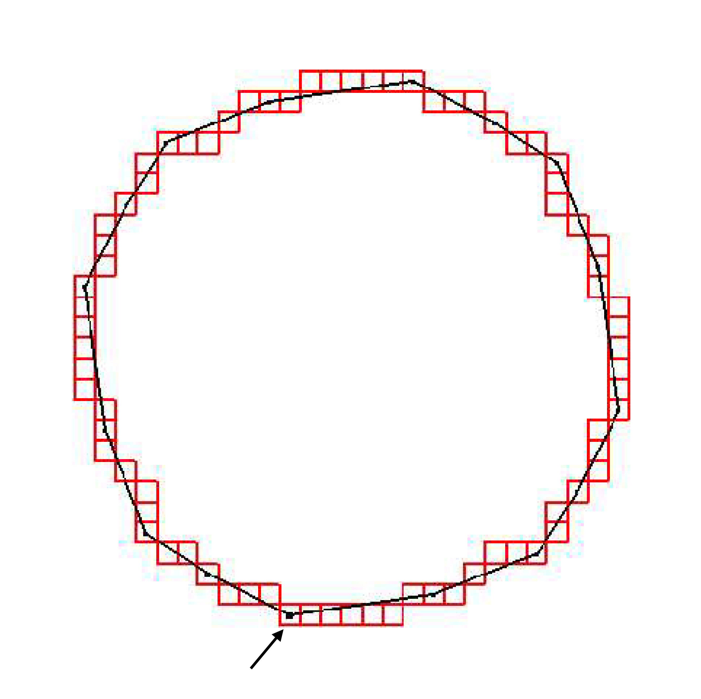
Given a digitization model:
Def.
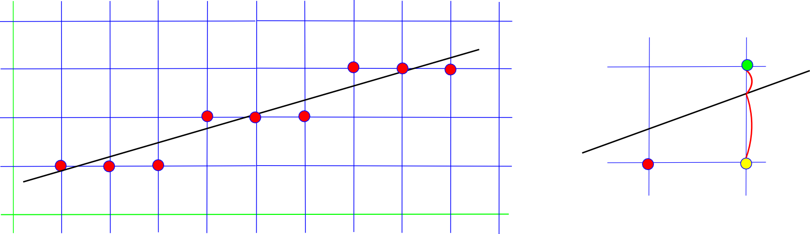
A digital straight line (resp. segment) is the result of a digitization and an Euclidean line (resp. segment)
Digital Segment tracing by Bresenham’s algorithm
GIQ based definition: For each abscissa we consider the closest grid point
Incremental construction
Properties
Segment between  and
and  in
in  with slope in [0,1]
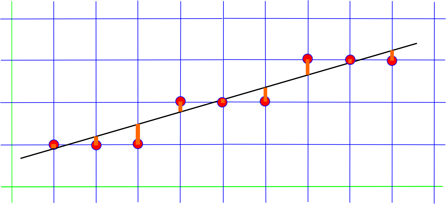
Naive approach
y = y_s
for(i = x_1; i <= x_2; ++i)
   display(i,y);
   y_real = (y_2-y_1)/(x_2-x_1) * (i+1) + y_1;
   dy = y_real - y;
   if ( dy > 0.5)
     y++;
e = x_2 - x_1
dx = 2*e
dy = 2*(y_2 - y_1)
while (x_1 < x_2)
  display(x_1,y_1);
  x_1 ++;
  e  -= dy;
  if (e <= 0)
     y_1 ++;
     e += dx:
Rationale
 inside the loop, 4 integer based operations and one comparison, no possible round-off errors
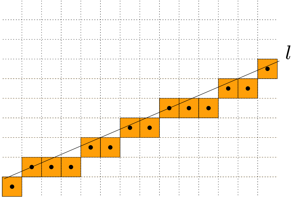
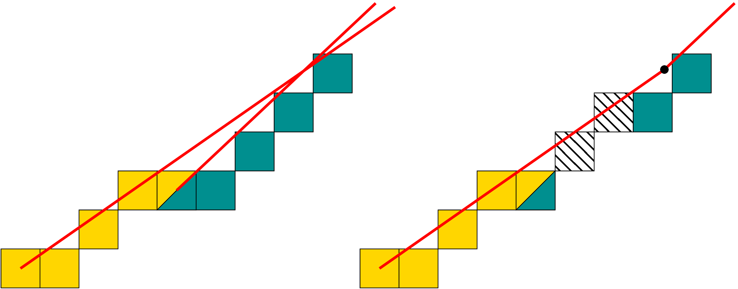
Let us consider GIQ digitization scheme (similar to Bresenham’s) and a straight line  with
with  . Let
. Let  be the digitization of the straight line and C its Freeman code
Thm

<demo>
Periodic structure  canonical pattern
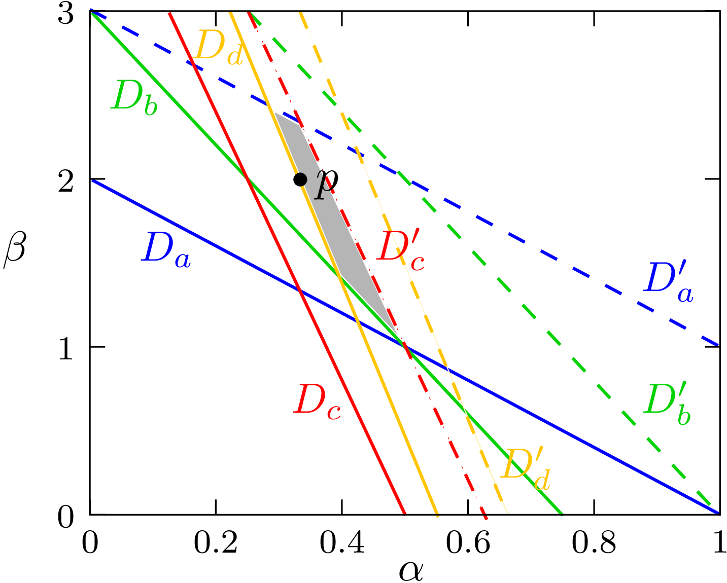
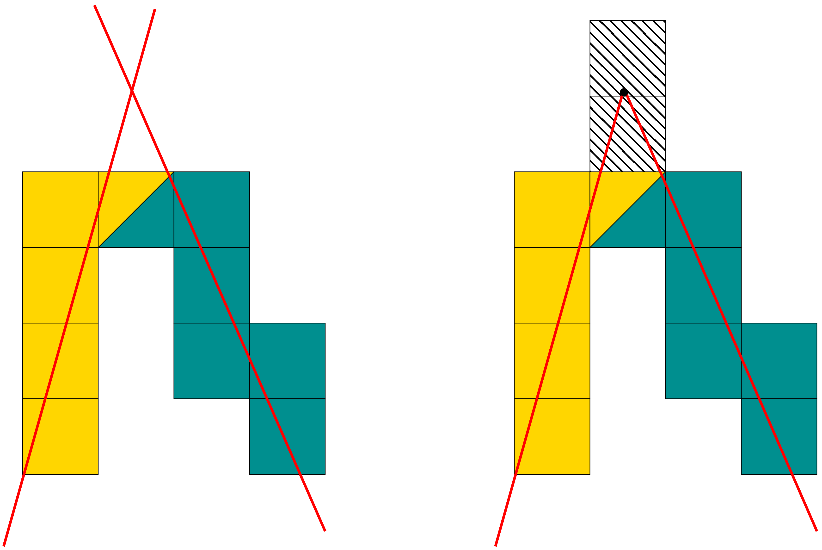
Any two points define a unique straight line
|

|
Two non-parallel straight lines intersects at a single point
|
Single point |
|
Empty set |
|
Non-connected set |
|
Connected set |
we need to redefine parallelism, intersections, …
Switching to another digitization scheme, we may avoid some situations.
E.g. with analytical models, empty set case will never occur
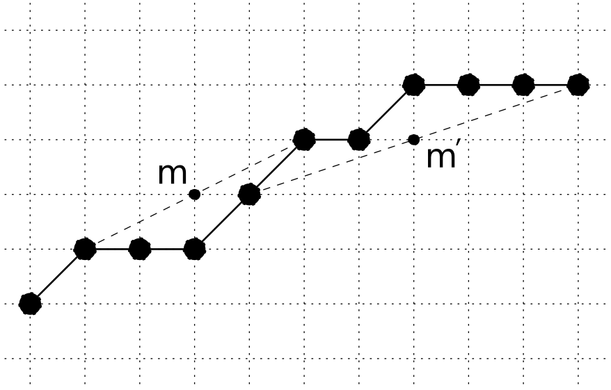
Chordal Property [Rosenfeld]
Def.
![\forall p \forall q\text{ and }\forall m\in[pq]\text{, there exists M(i,j) such that }\max(|i-x|,|j-y|)<1](_images/math/96b80543677750a4a8c85c446bf0b1172dbe1346.png)
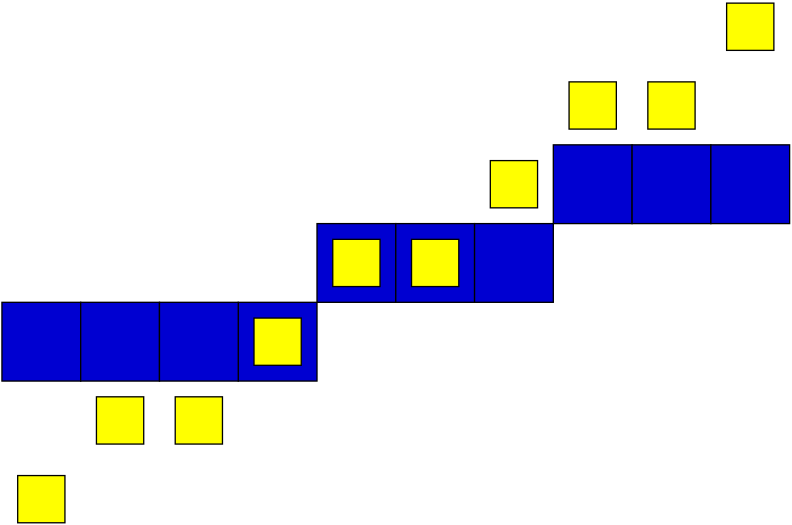
Evenness Property [Veelaer]
Def.
![\forall a,b,c,d\in[pq] \text{ such that }\vec{ba}_x=\vec{dc}_x,\, |\vec{ba}_y-\vec{dc}_y|=1](_images/math/804998660a4ebf9612c813ebb3140797fba58e0e.png)
Definition
Def.
Diophantine equation = Equation with integer parameters and solutions in 
Example
(with  )
)
What is the general form of solutions of such linear diophantine equation ?
 , and let denote the solutions
Existence
Homogeneous case
General case

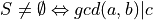
Since  ,
,  such that
  [Bezout]
Your turn: 12x+15y=51
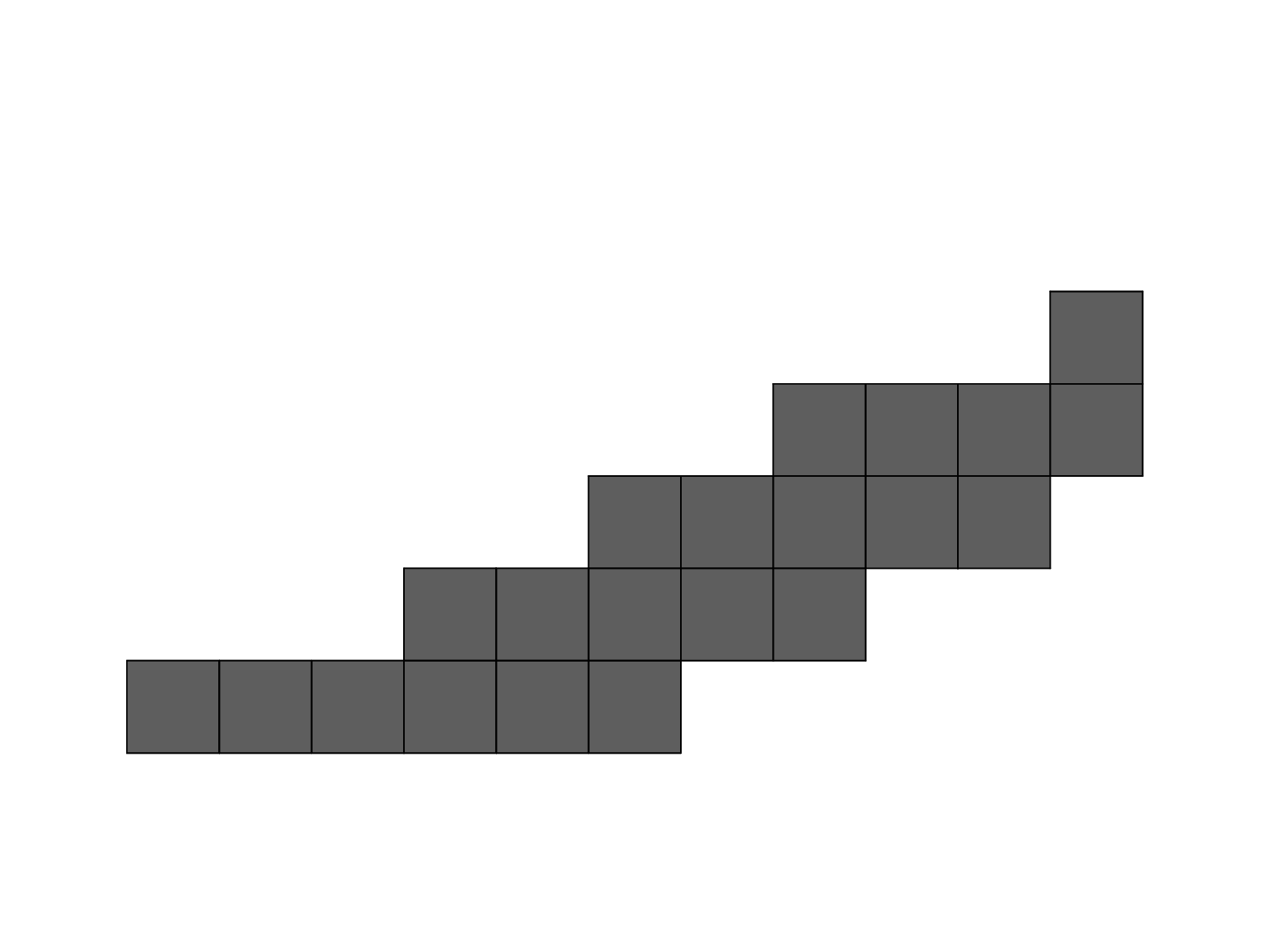
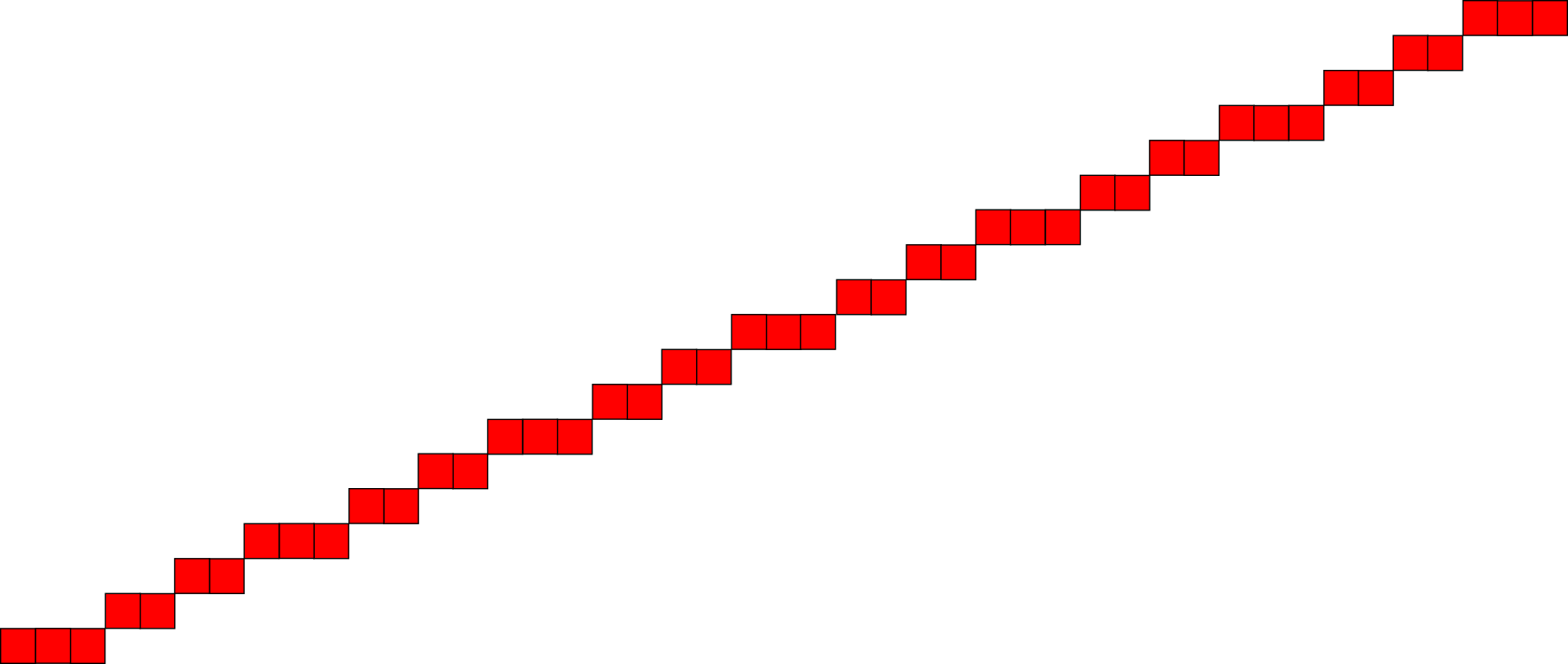
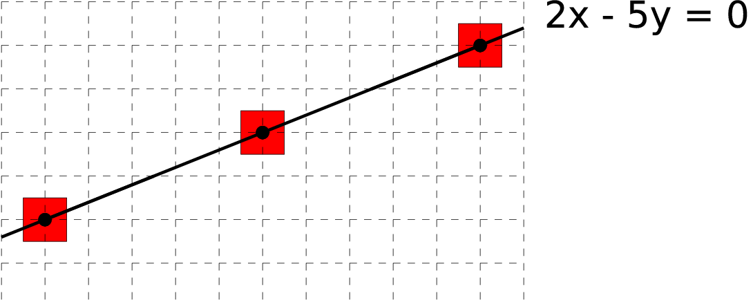
Idea Design a analytical definition instead of combinatorial ones
Def.
 is a analytical DSS with parameters
  with
with  , if for all
  , we have
 acts as a thickness (arithmetical thickness, >1)
 is the DSS slope
 is the arithmetical intercept
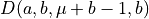
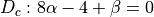
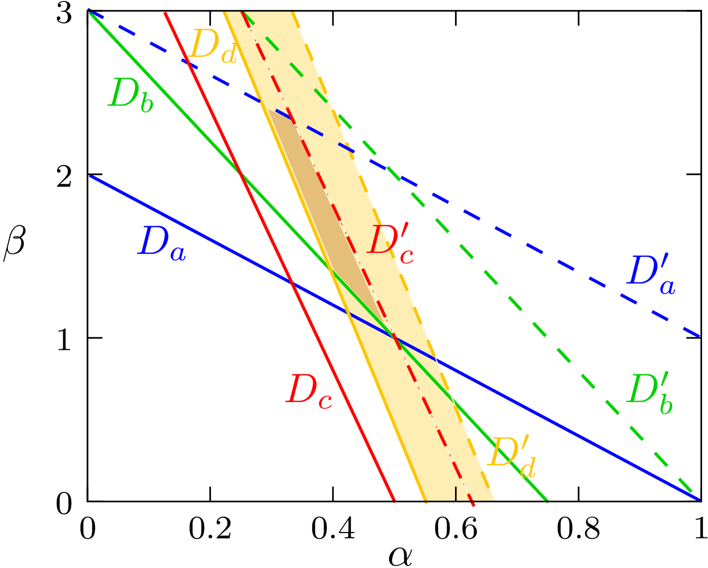
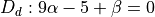
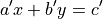
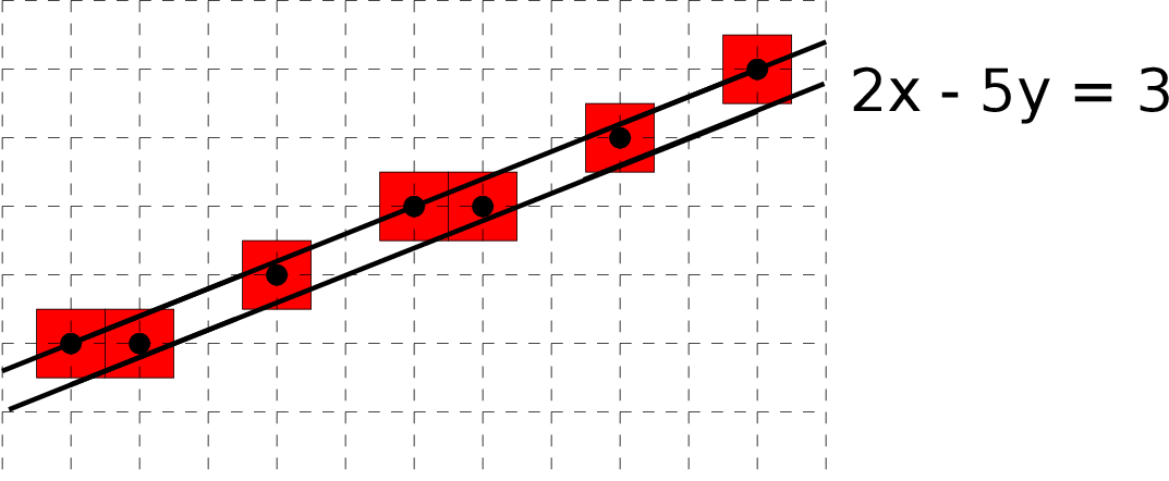
S is the union of solutions of  diophantine equations:
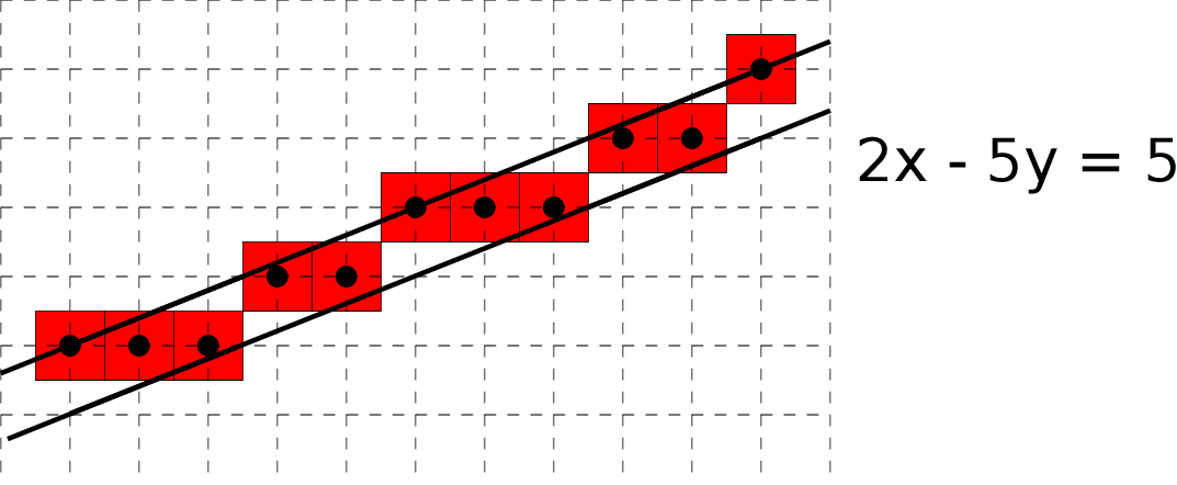
Thm.

 , D is not a (k)-path
 , D is a (0)-arc
 , D is a (1)-arc
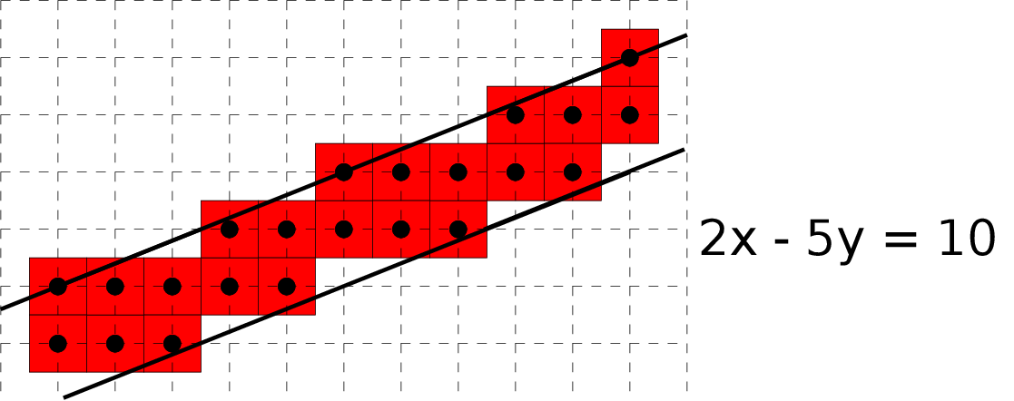
 , D is (*)-connected
 , D is thick
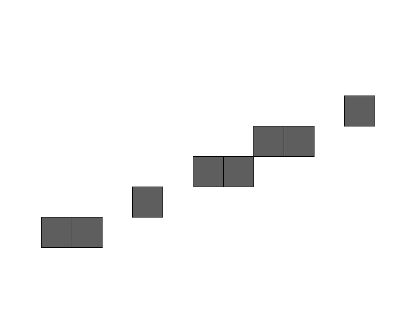
|
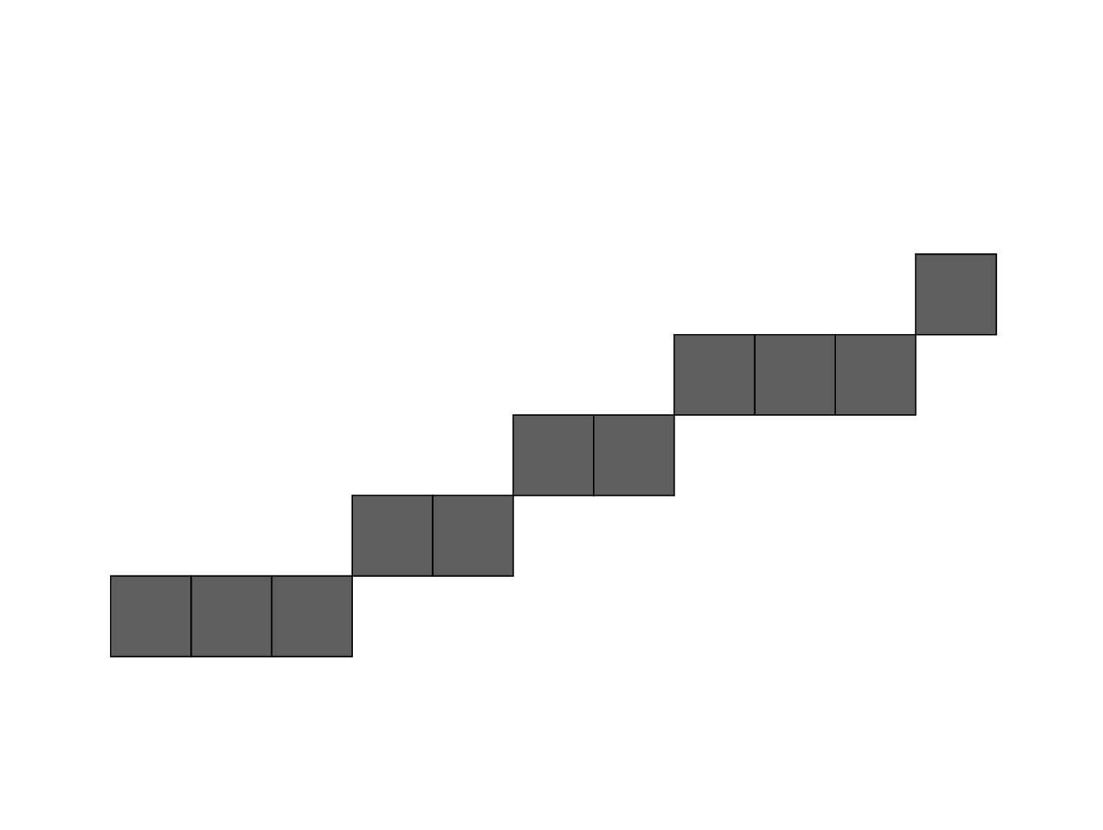
|
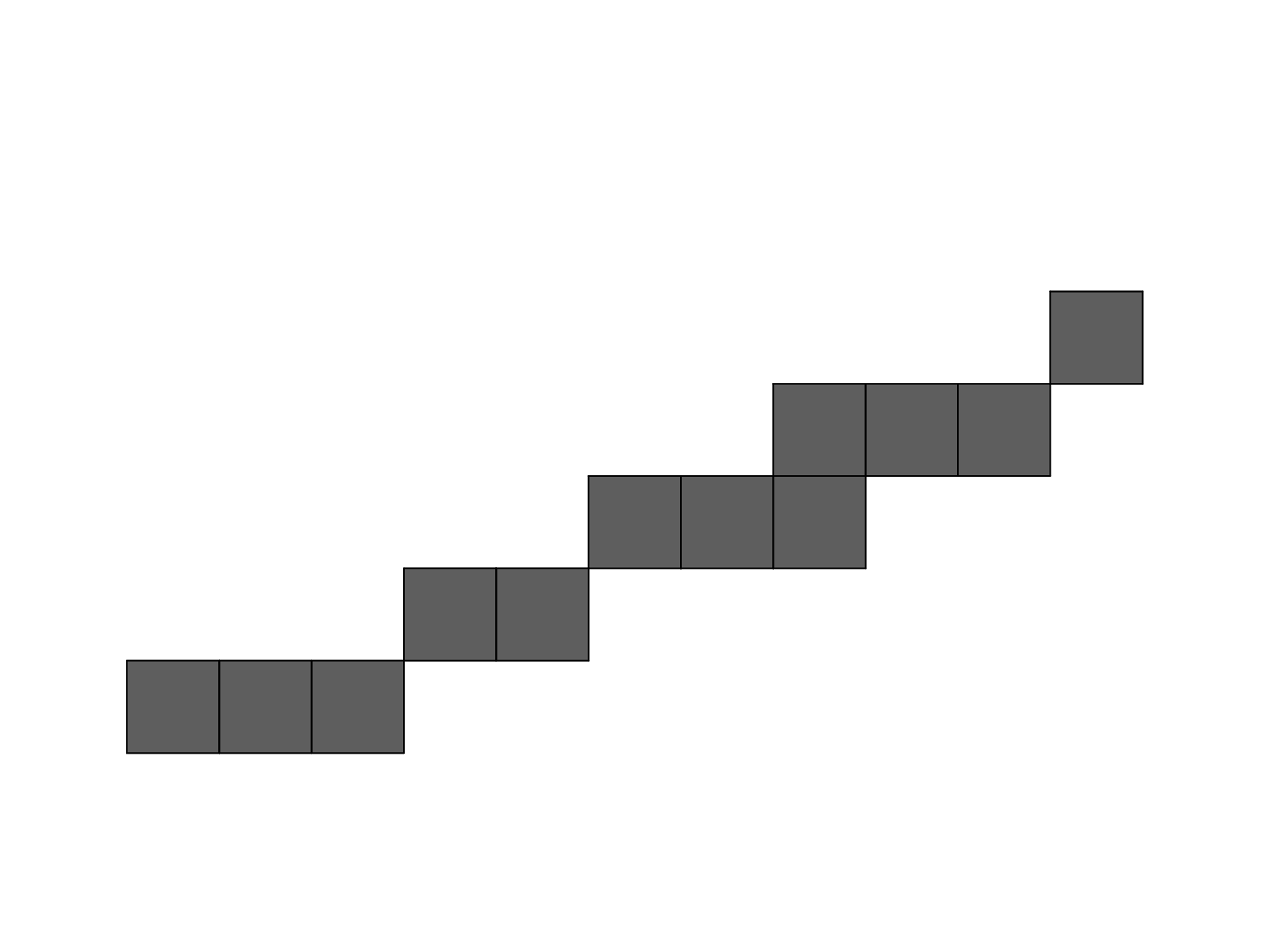
|
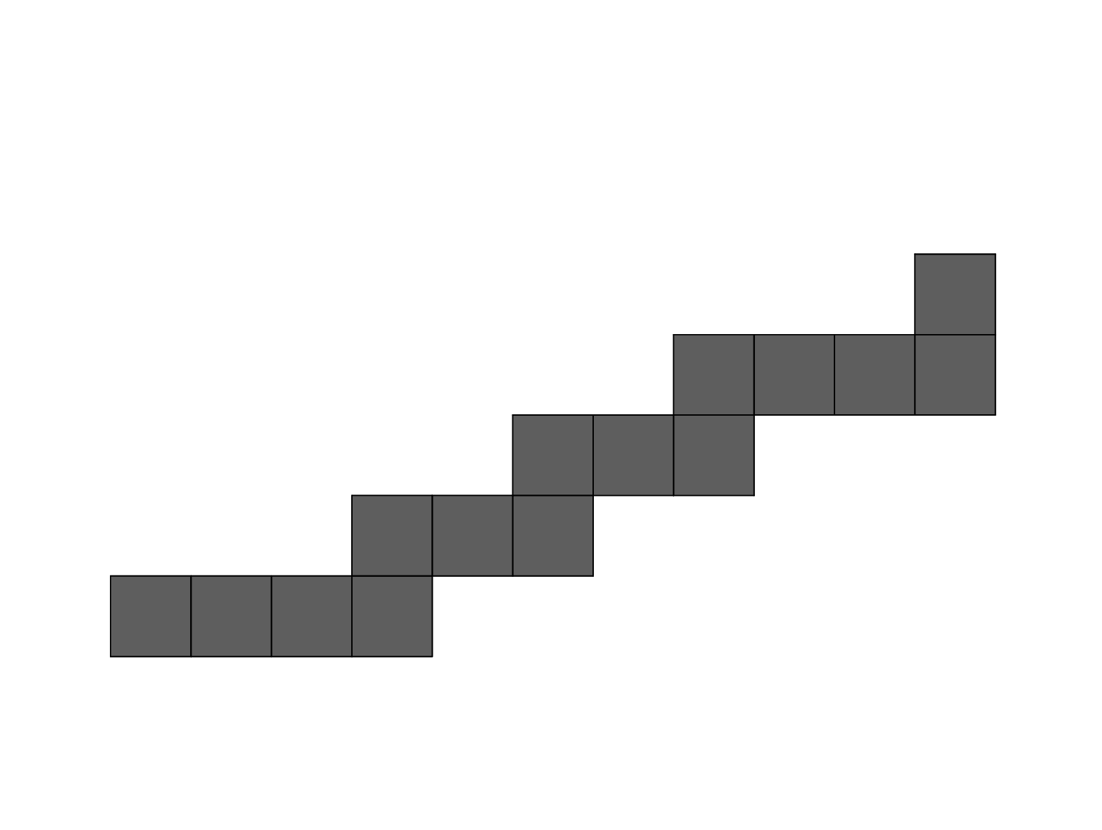
|
|
| D(3,7,0,5) | D(3,7,0,7) | D(3,7,0,8) | D(3,7,0,10) | D(3,7,0,16) |
Given an Euclidean straight line 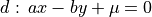 with
with  Without loss of generality, we suppose
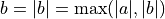
 corresponds to a kind of OBQ of d
 corresponds to a kind of BBQ of d
![D(a,b,\mu+[\frac{b}{2}],b)](_images/math/61290f76c2bcaf351af5bf128a07c49636d64f25.png) corresponds to the GIQ quantization of d
corresponds to the GIQ quantization of d
![D(a,b,\mu+[\frac{a+b}{2}],a+b+1)](_images/math/8b747b019e0e32965b60d4677f263ddc9846605c.png) corresponds to the supercover digitization of d (analytical digitization with squares)
corresponds to the supercover digitization of d (analytical digitization with squares)
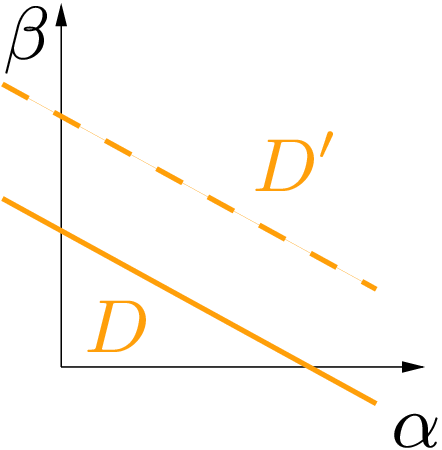
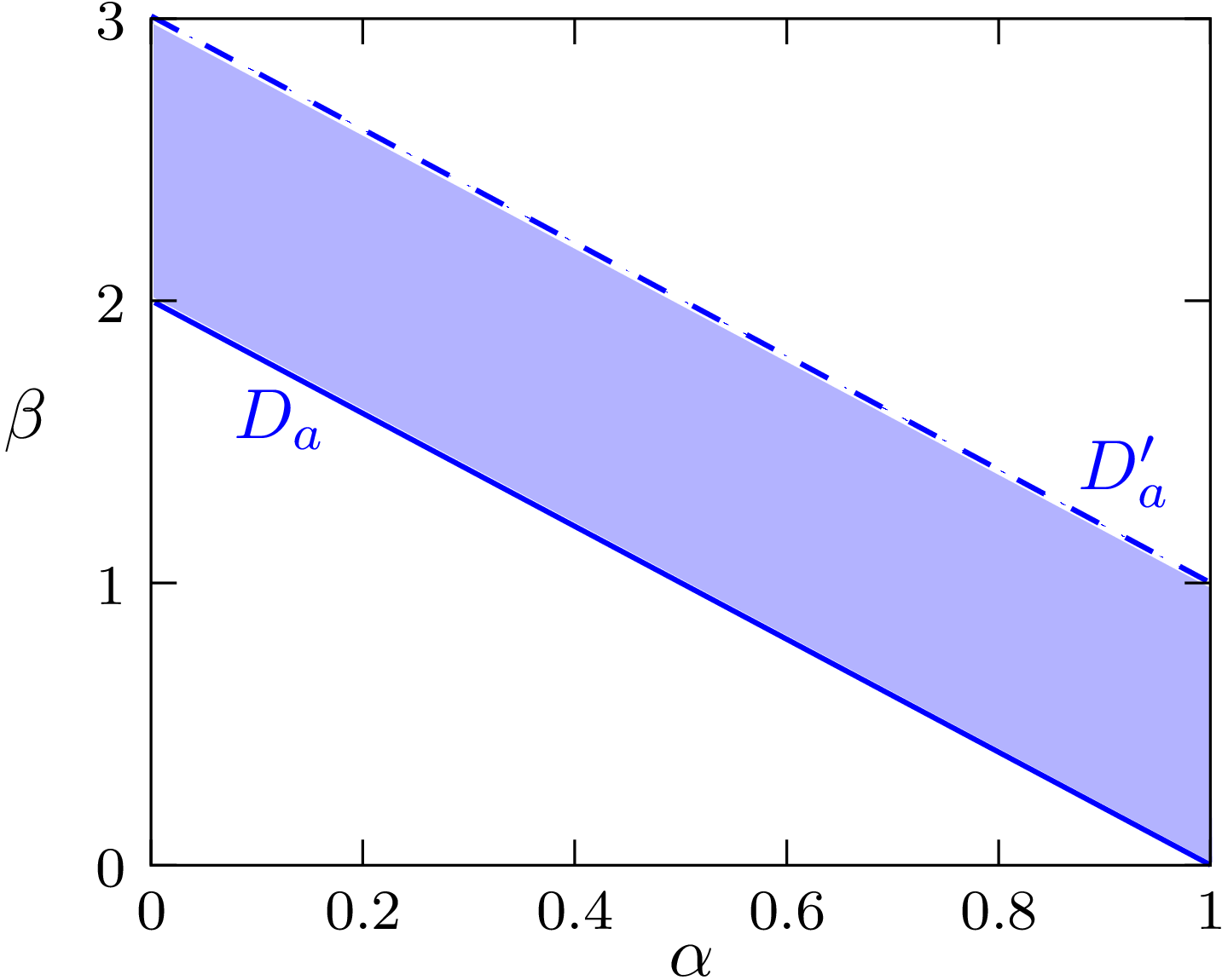
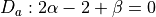
Thm.
Given , D is invariant by translation with vector  (
( )
)
<proof>
Corollary
Coro.
Any sequence of  pixels defines a DSS pattern, the pattern is minimal iff
Similar results than the one obtained by straight segment digitization but more generic
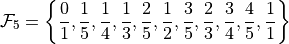
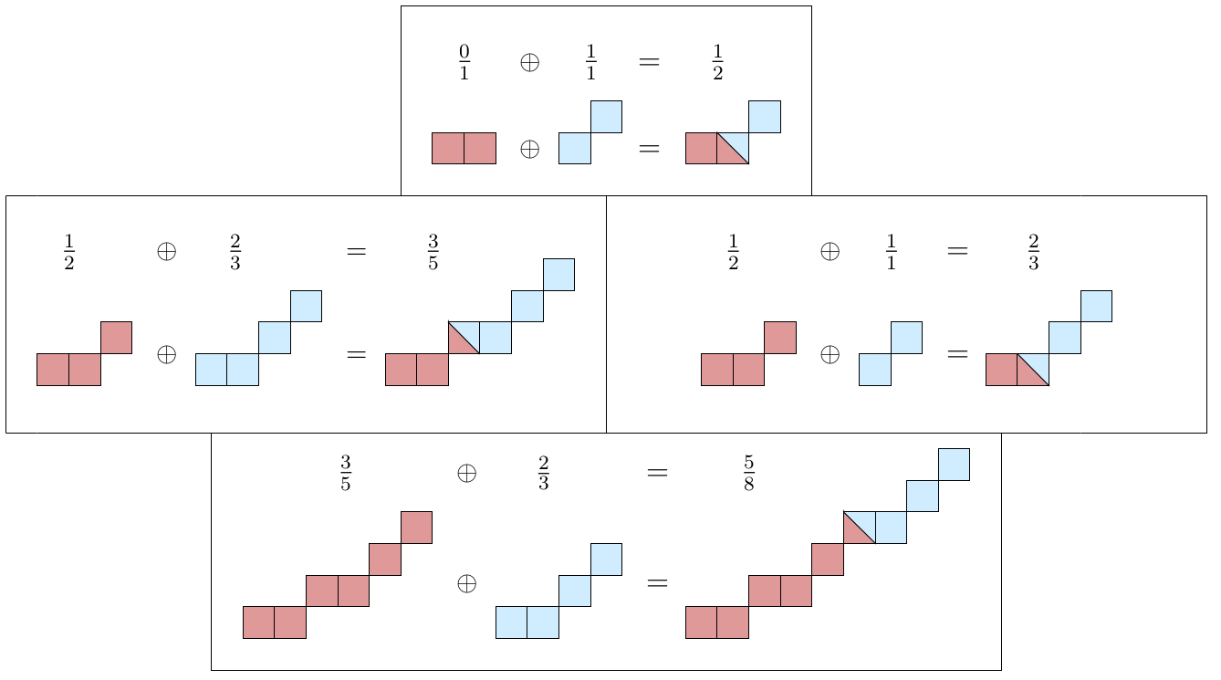
Def.
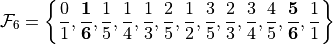
The Farey Series  of order m is the ordered sequence of irreducible fractions with denominator less or equal to m
Properties
 et
et  are two successive fractions in (with
  ), then
 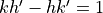 ,
,  and are three successive fractions in (with
  ), then
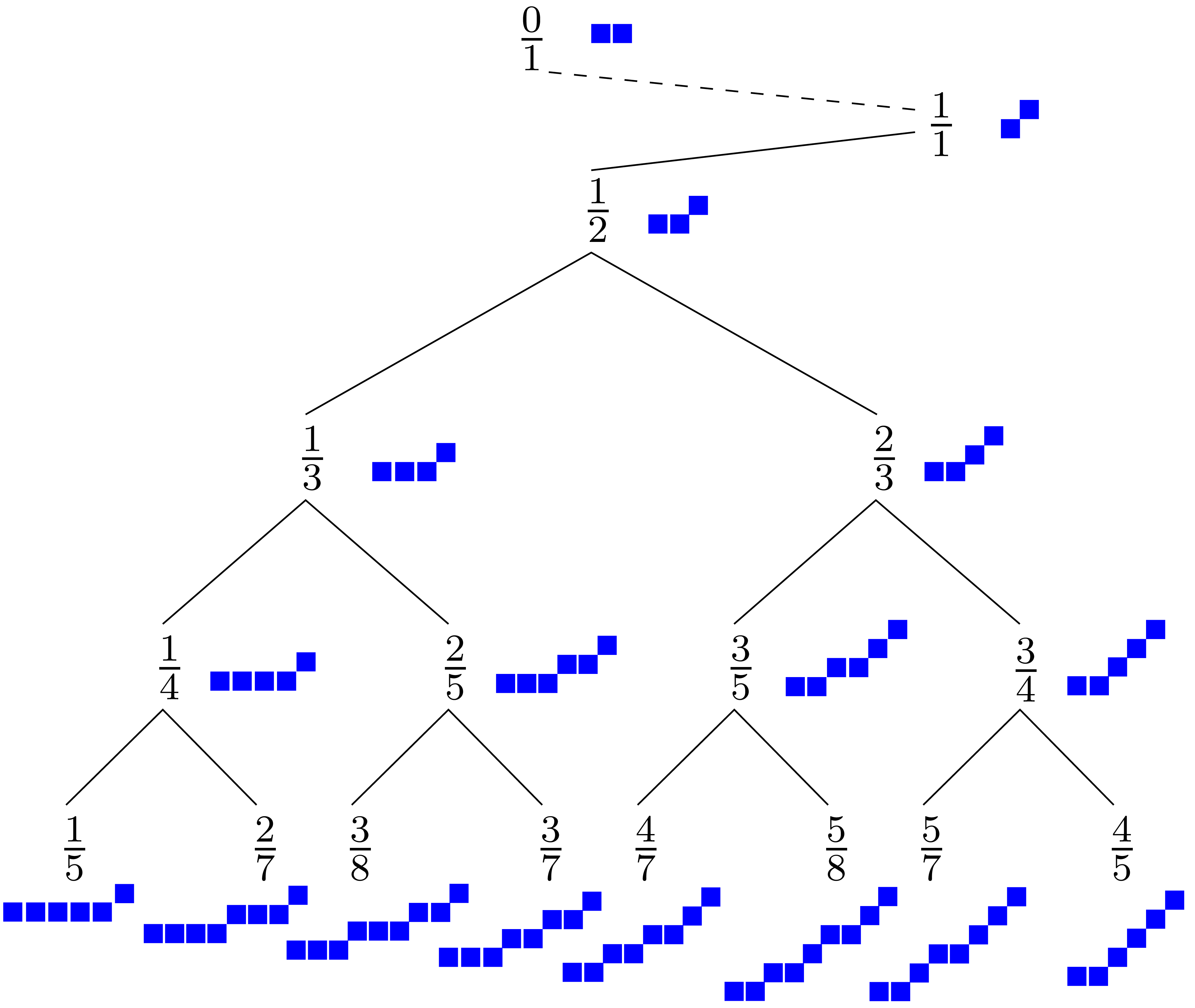
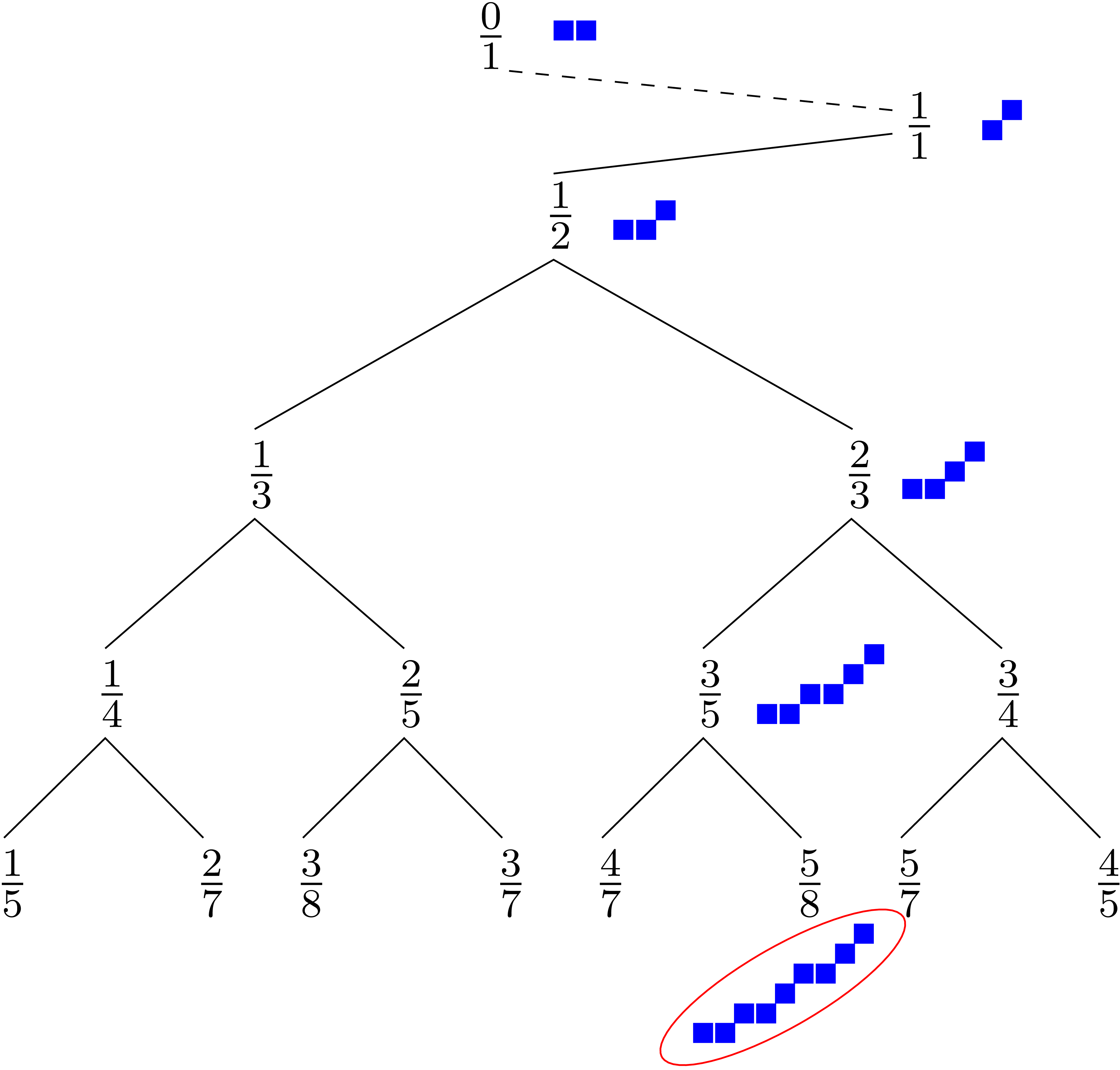
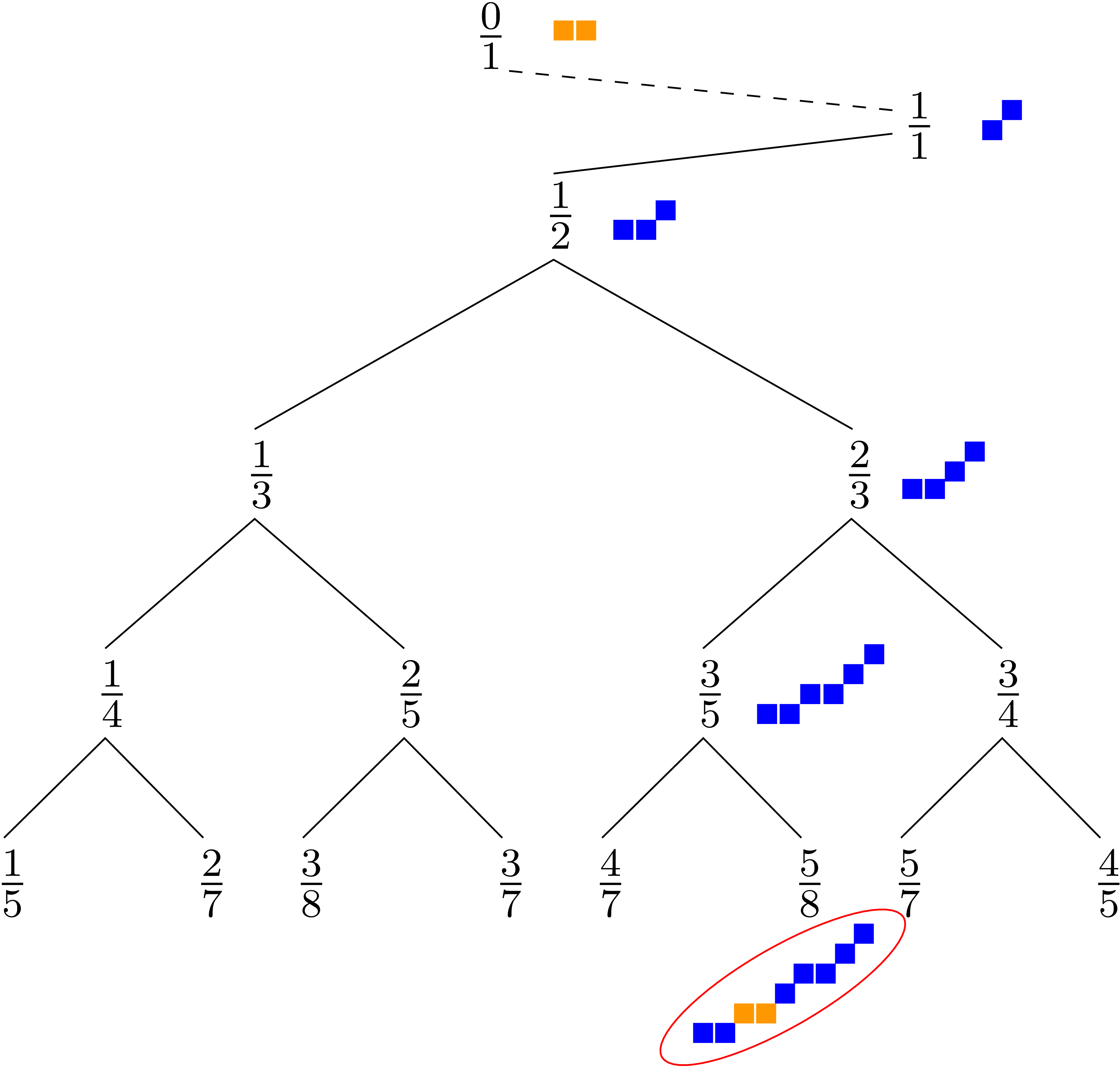
  (median fraction)
 is given from inserting median of successive fractions with denominator
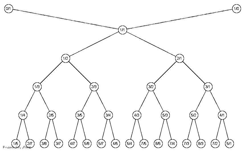
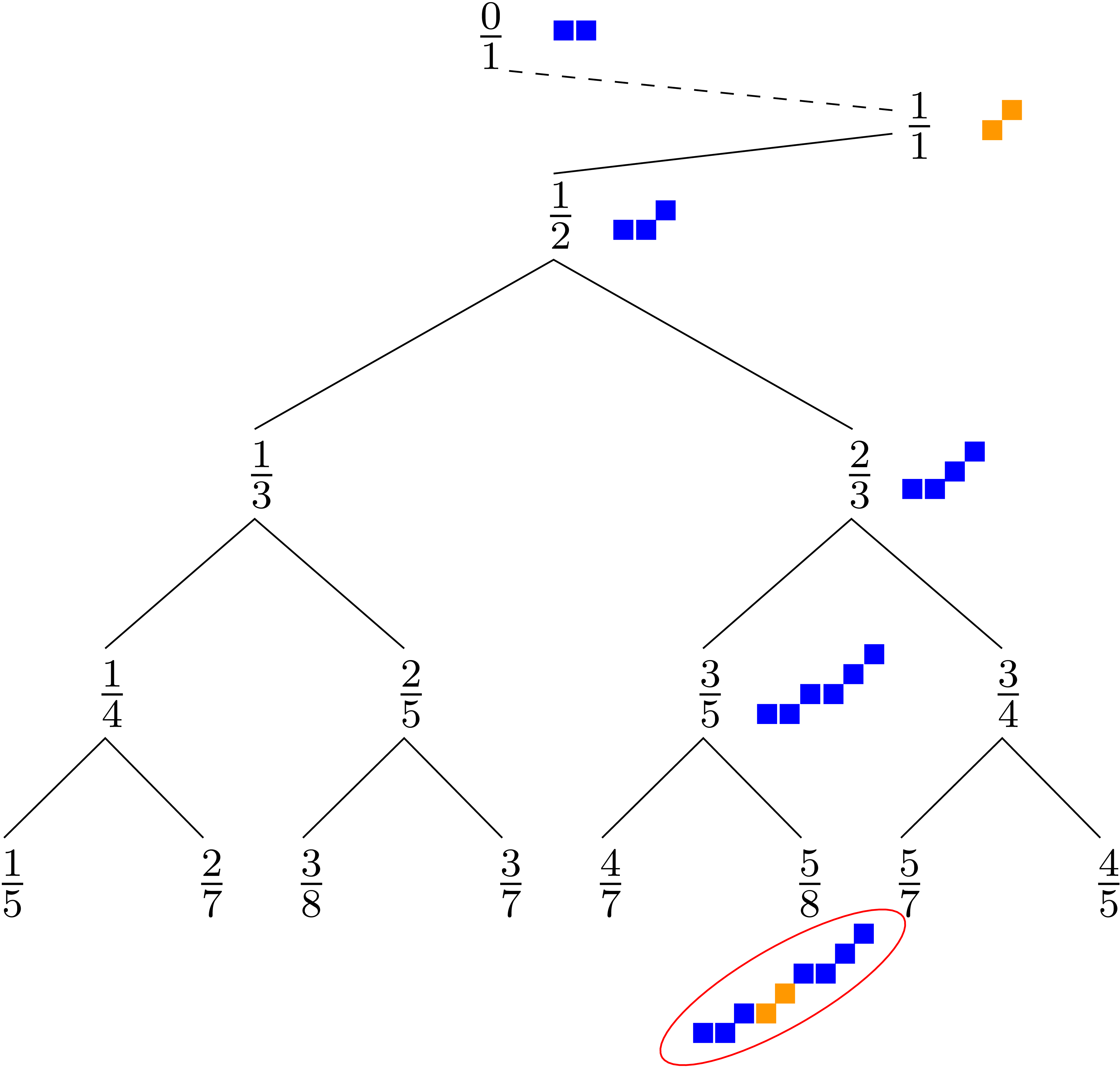
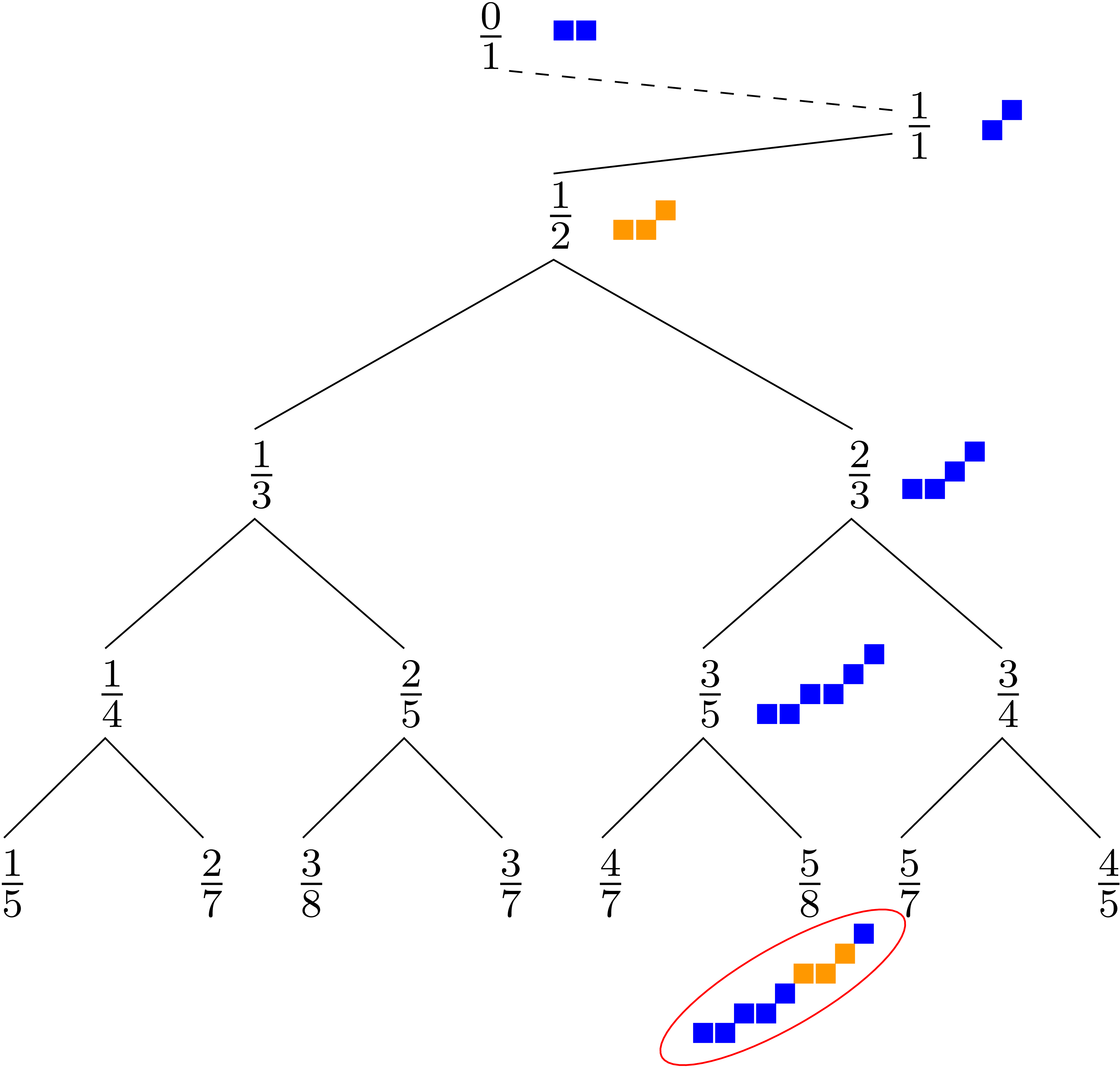
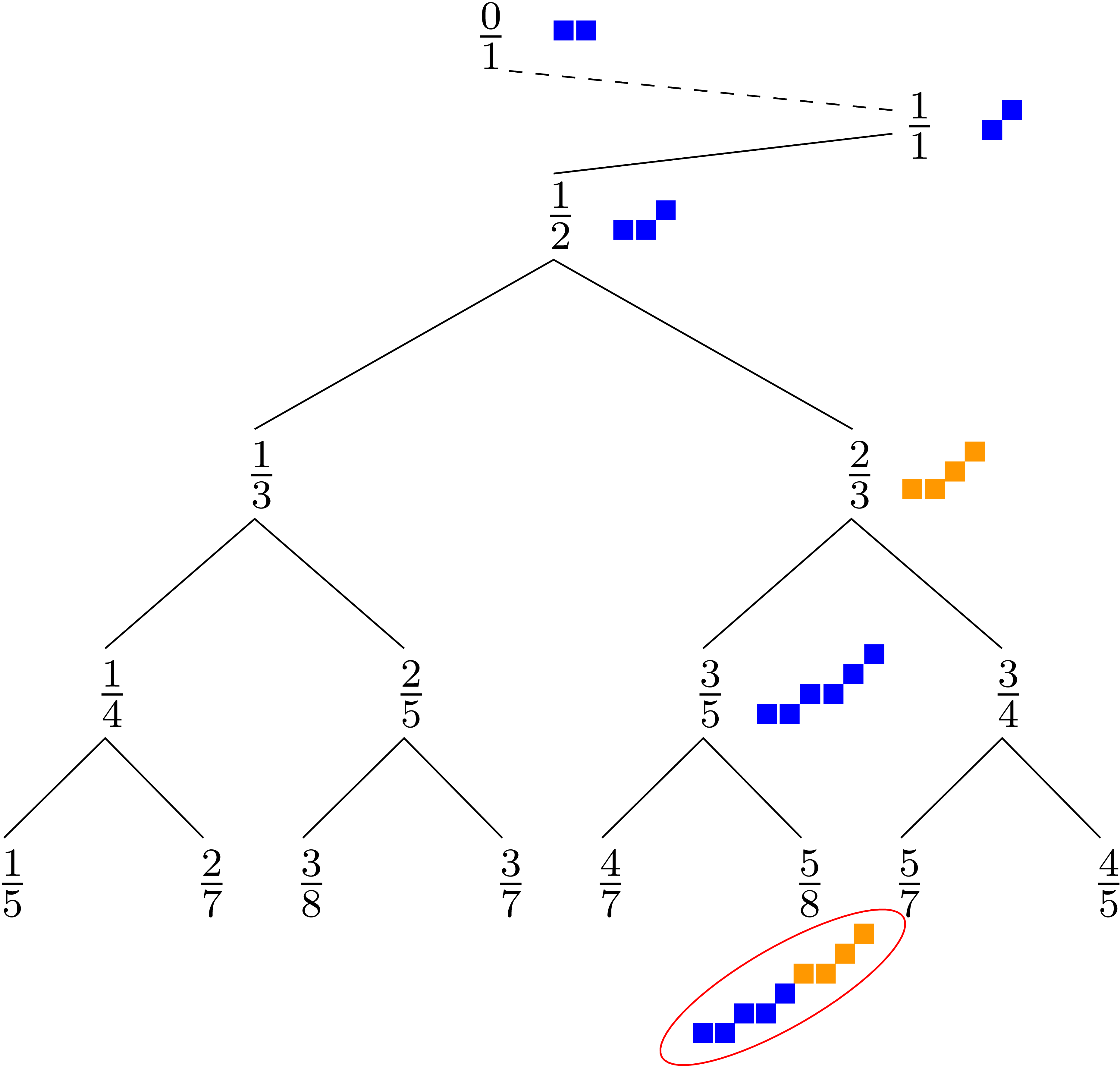
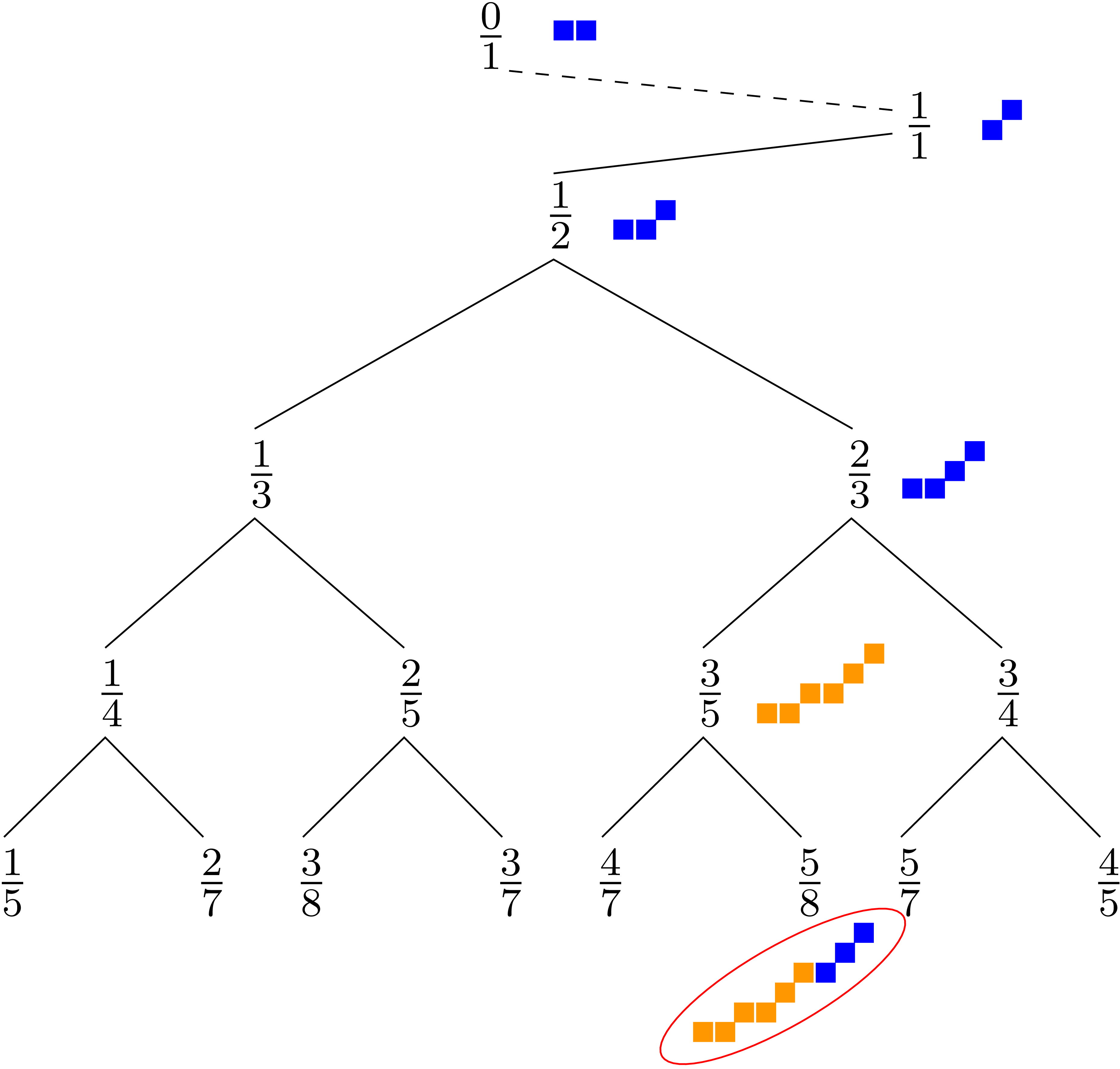
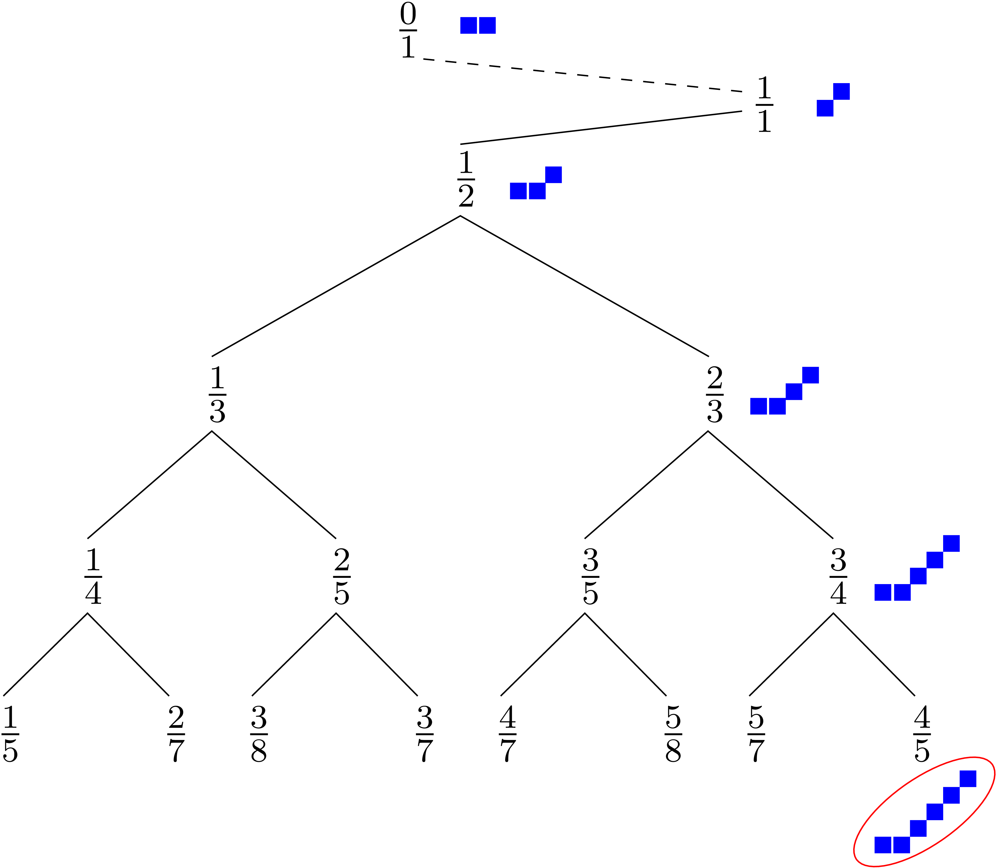
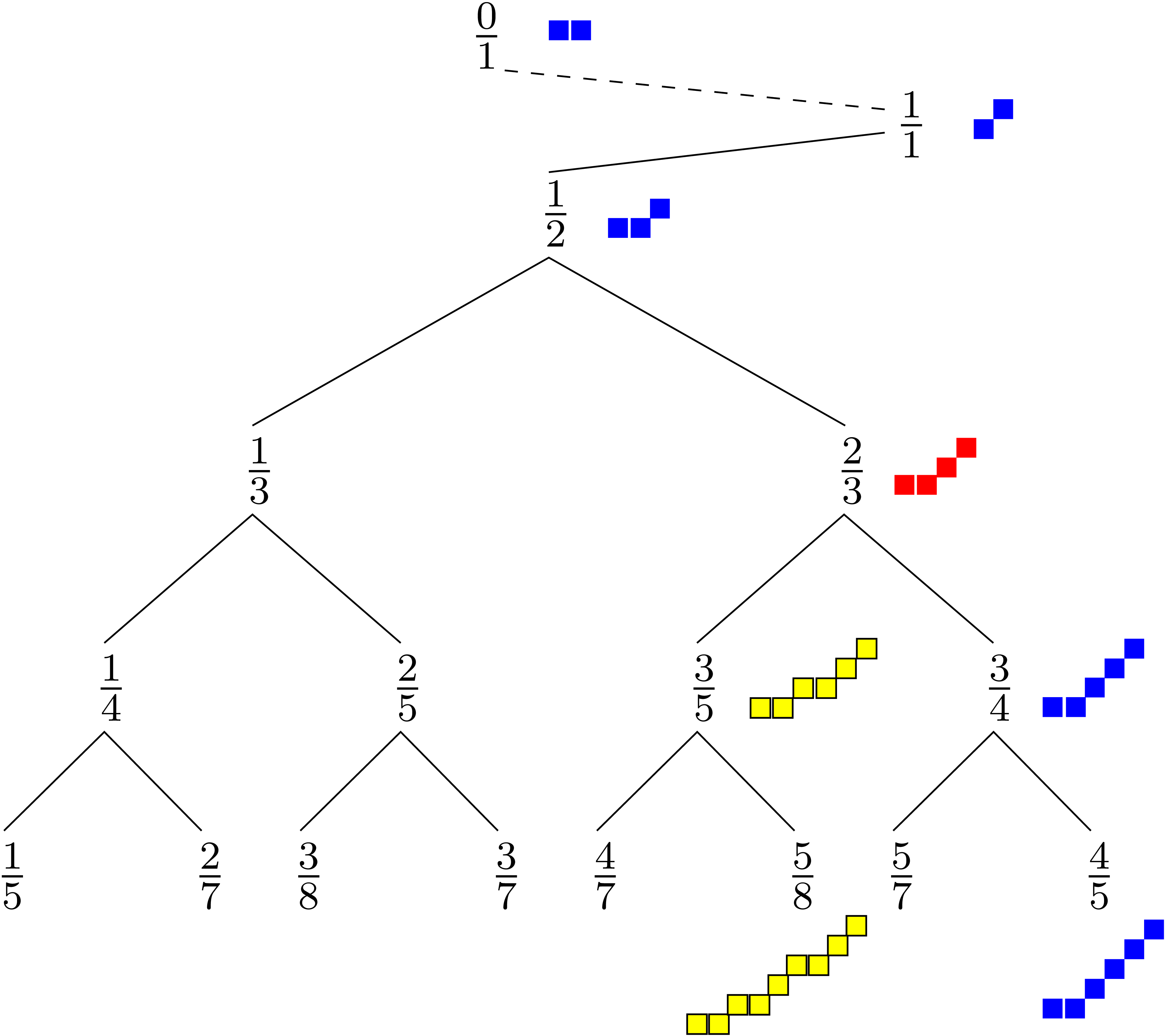
Binary search tree on fractions
Given
 with slope
  and Freeman code of one of its pattern
 with slope
  and Freeman code of
one of its pattern
and Freeman code of
one of its pattern 

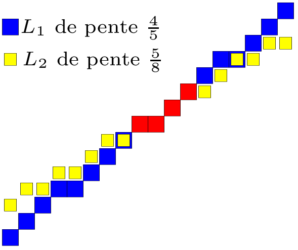
 (unimodularity)
Then
 is the Freeman code of one period of the DSS with slope
Idea
Given a digital set , and a geometrical primitive (DSS,
Digital circle, digital plane, …), decide if is a subset
of such primitive
Detection Yes/No answer
Recognition a valid parametrization of the primitive, the complete set of primitives containing -> preimage
Useful to
Idea
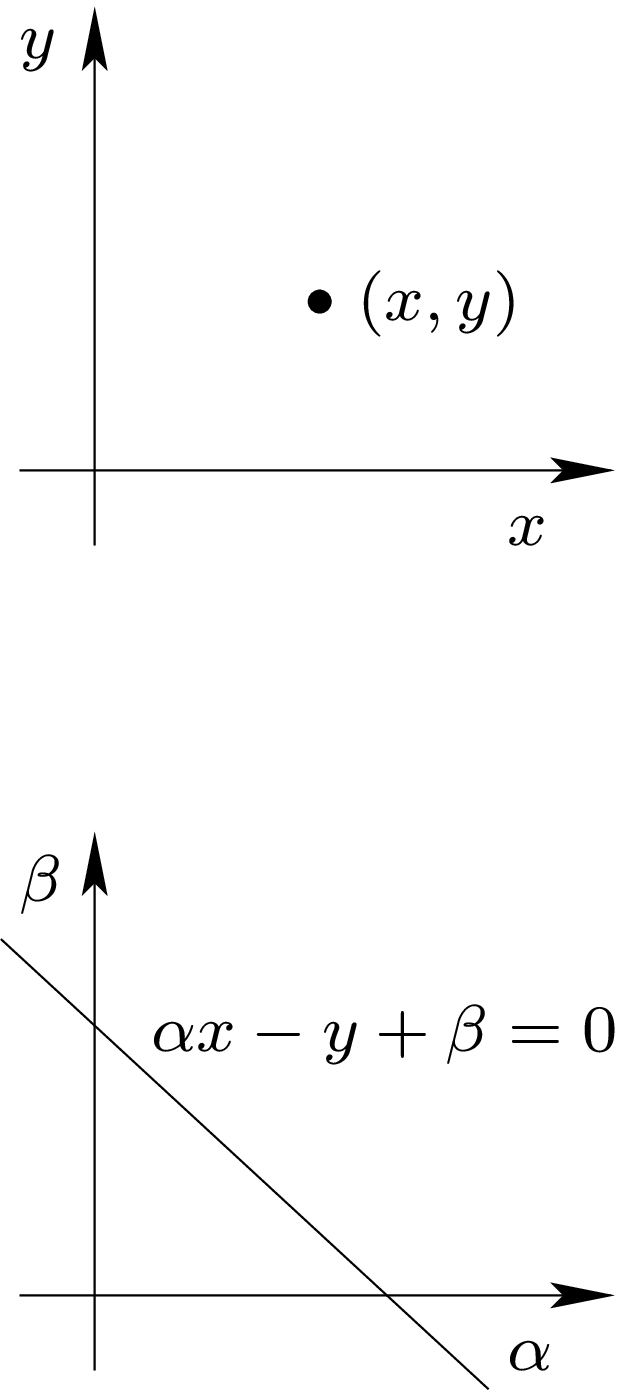
Revert the digitization process and solve a dual problem
DSS: Linear dual space

|
|
|
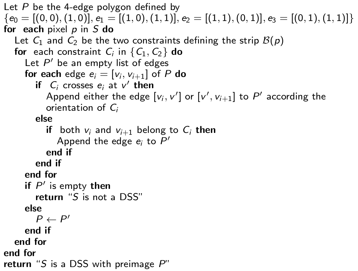
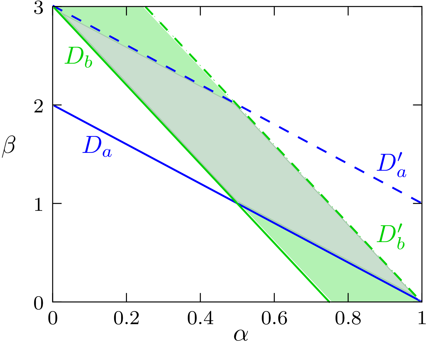
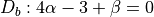
Let us consider the following OBQ digitization scheme of 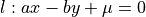
Each pixel  contributes to two linear constraints:
|
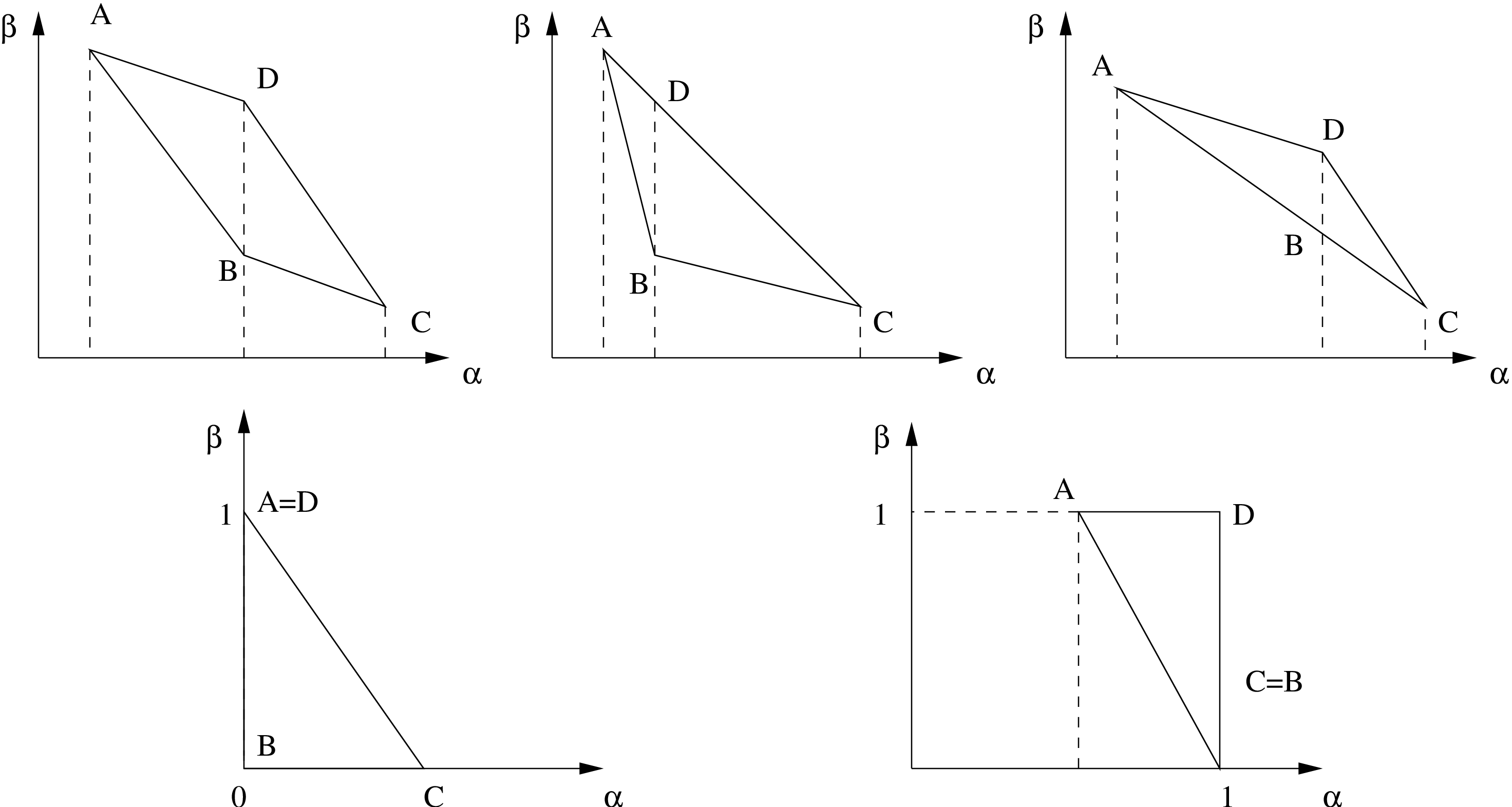
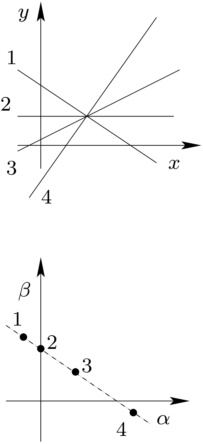
Algorithm principle
Given a set S of pixels
 (i.e. we consider DSS in the first octant) and the two associated constraints
 if is empty, S is not a DSS (for OBQ scheme)
is called the preimage of S
|
 ,
,  and
and 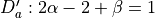
|
 ,
,  and
and 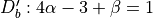
|
 ,
,  and
and 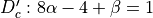
|
 ,
,  and
and 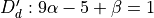
|
 in the dual space leads to
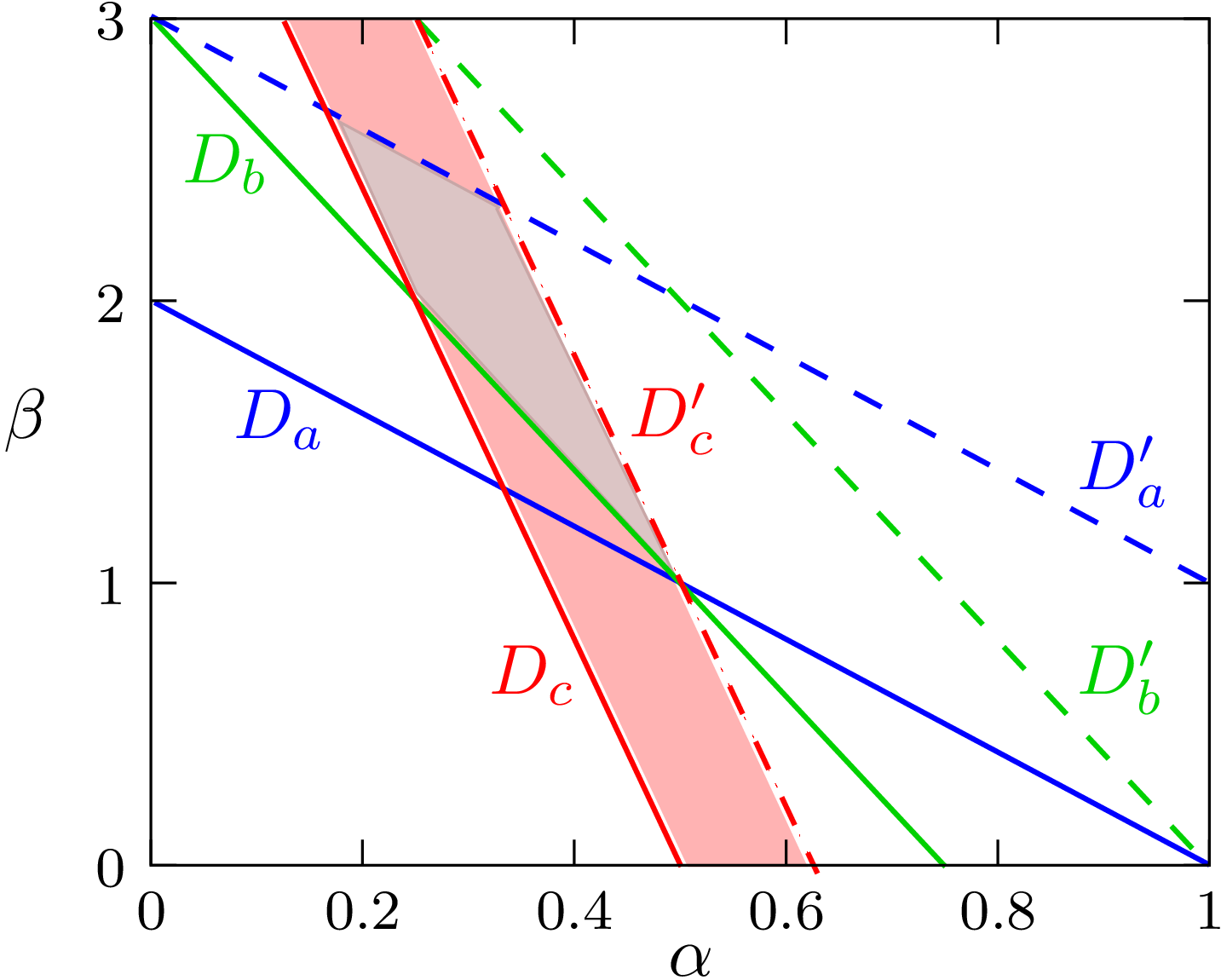
Preimage = Classical linear programming problem
is convex to maintain (
 per constraint)
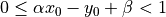
If is a (0)-path
Thm.
has at most 4 vertices in the dual space
On-line DSS recognition in (O(1) per constraint)
Farey Fan
The Farey Fan of order  is a decomposition of the space into cells where each cell corresponds to a DSS preimage of length
|
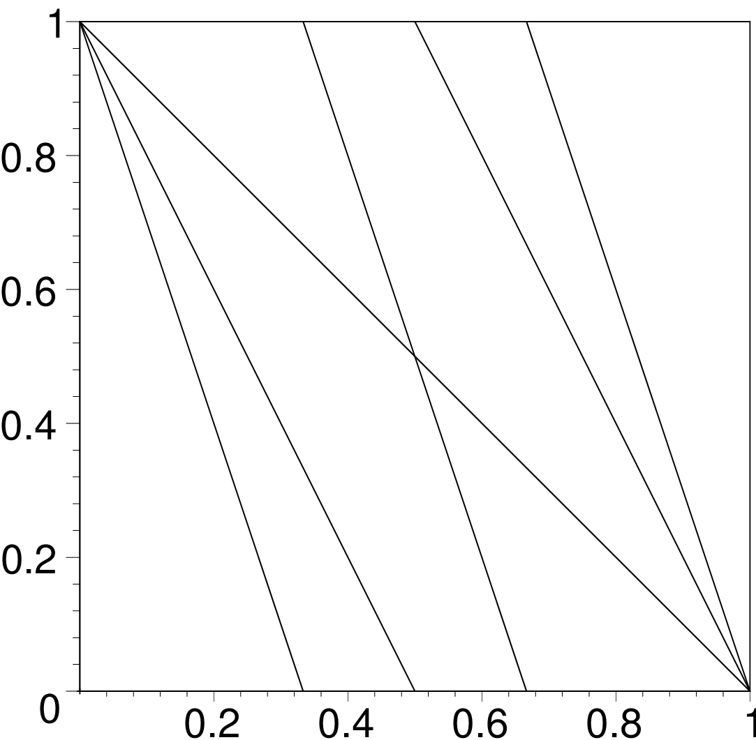
|
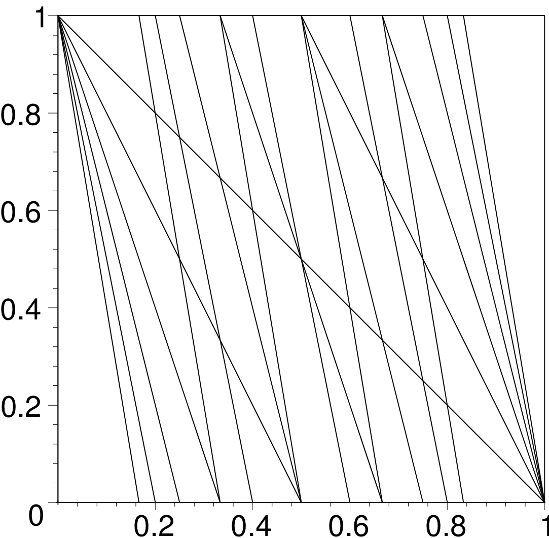
|
| Order 2 | Order 3 | Order 6 |
Idea
Use the analytical representation of DSS:
 a DSS in the first octant
the reminder of a pixel  is the quantity

the k-th net is defined by the solutions of
the DSS is the union of nets with 
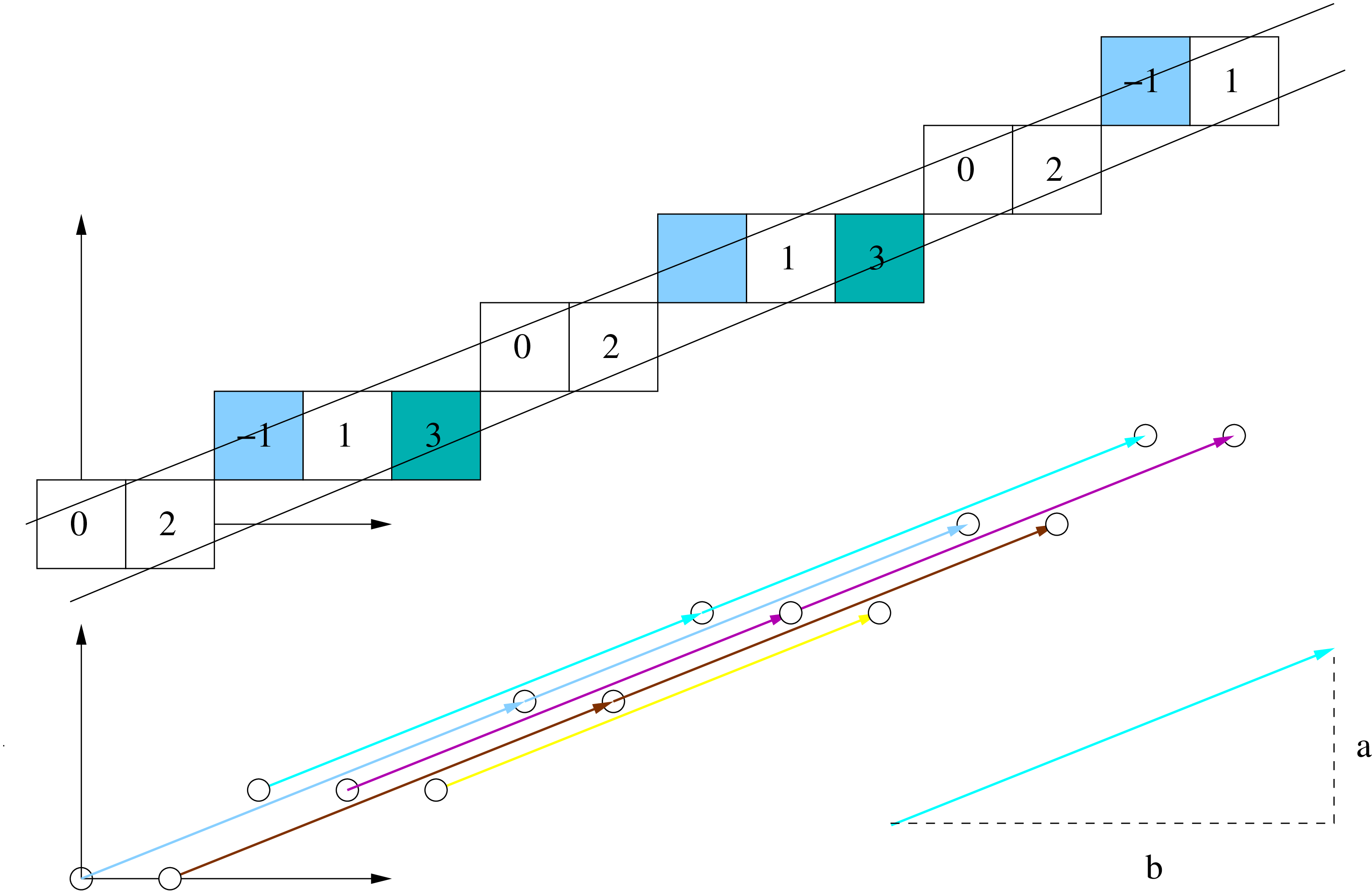
Definitions (again)
Defs.
is exterior to D if its reminder is lesser than  or greater than
  is weakly exterior to D if its reminder is equal to or is the upper leaning net
 is the lower leaning net
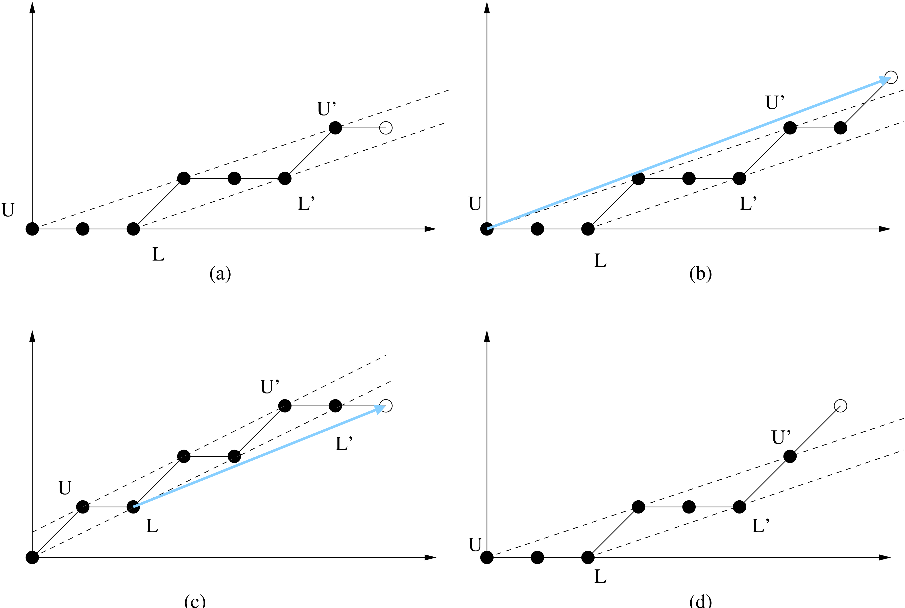
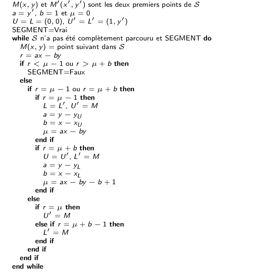
Let U (resp. U’) be the upper leaning point with minimal abscissa (maximal abscissa) and L (resp. L’) be the lower leaning point with minimal abscissa (maximal abscissa)
Given a DSS digital set S w and a point M (with reminder r), we have to decide if  is still a DSS
Thm.
 then is a DSS with parameter cannot be a DSS
 , is a DSS where the slope is given by
 , is a DSS where the slope is given by
At each step, we maintain/update U,U’,L,L’ and DSS parameters a,b,
Computational cost
algorithm with  per pixel
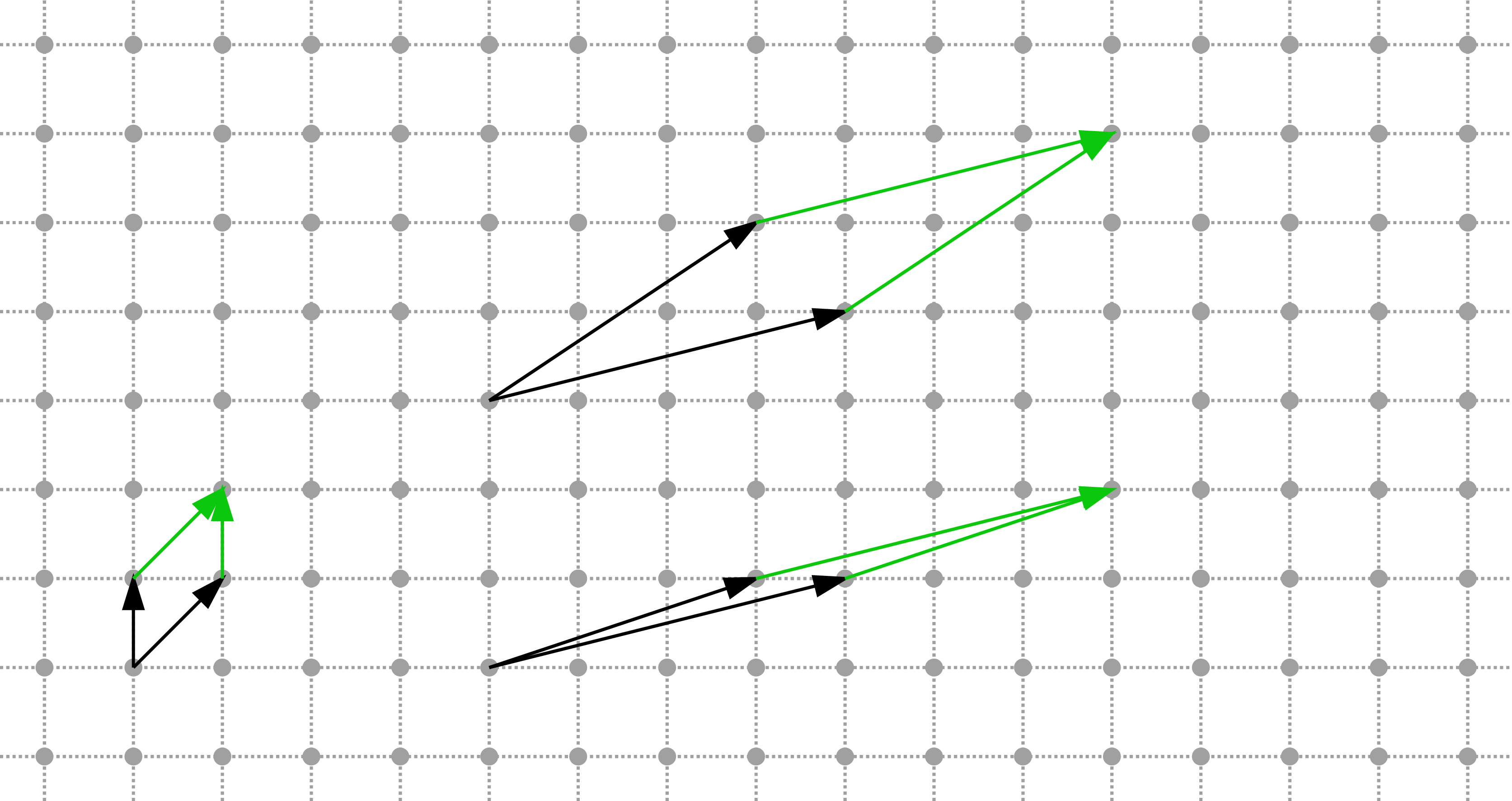
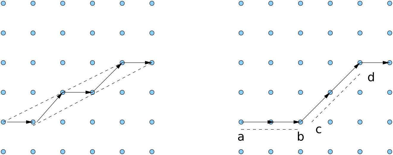
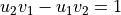
Key point of the proof: unimodular vectors
Given two vectors  ,
,  and
and  are unimodular iff
E.g.  and are unimodular if
  is weakly superior
(if vectors define fractions, fractions are neighbors in a given Farey series)
Unimodular means that there is no integer point in the parallelogram ( )
)
Similar approaches
 with similar topological results according to , with similar arithmetical structure (leaning points, unimodular vectors, …)
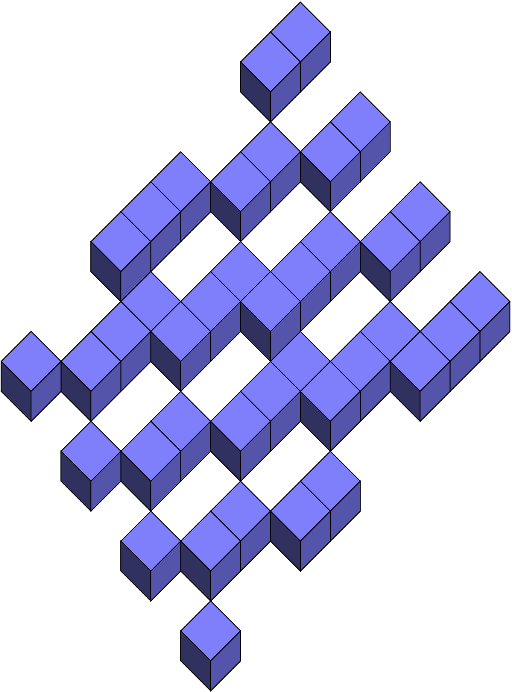
|
|
|
| P(6,13,27,0,15) | P(6,13,27,0,27) | P(6,13,27,0,46) |
Digitization -> Constraints
Given the primitive (plan, circle, …), digitization usually implies inequality system we have to solve
Usually:
Regularity/arithmetic in analytical representation
Design the recognition as a separation problem with tools from Computational Geometry
In practice: a kind of mix between all these approaches…
Idea
Starting from a contour point (and given a direction), decompose the contour into maximal DSS adding pixels one by one
|
|
|
O(n) algorithm
Changing the starting point, decompositions differs by one (N, N+1)
Similar approach but
Usually
|
|
Principle
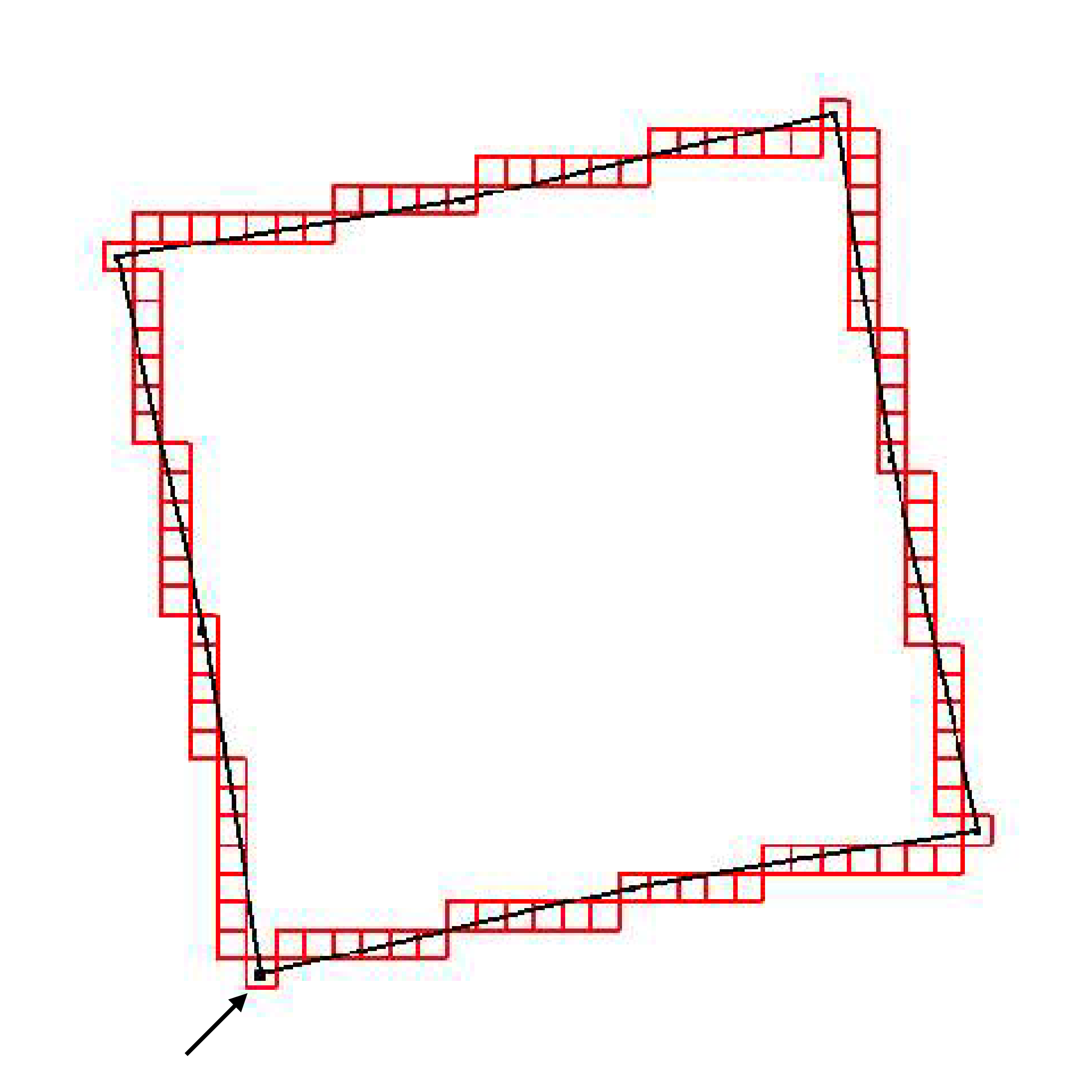
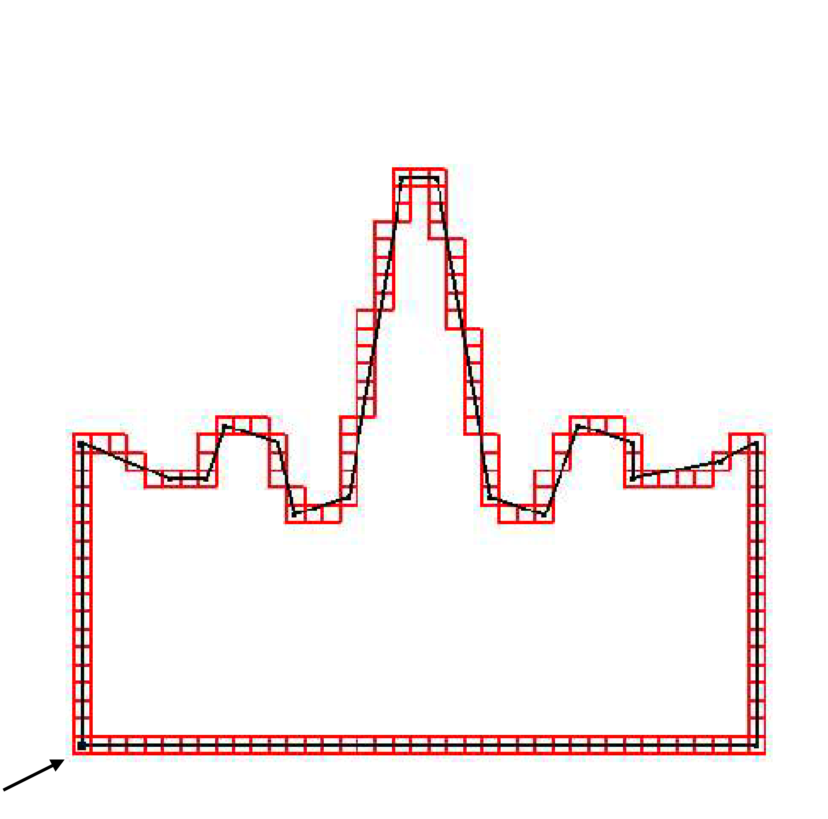
Convert a digital contour into a polygon such that its digitization is the input digital set
First approach: use DSS decomposition
Indeed, DSS segments are “reversible” … but not the vertices..
|
|
We need to constraint the preimages to ensure that successive DSSs have euclidean representative segment with “reversible” intersection vertex
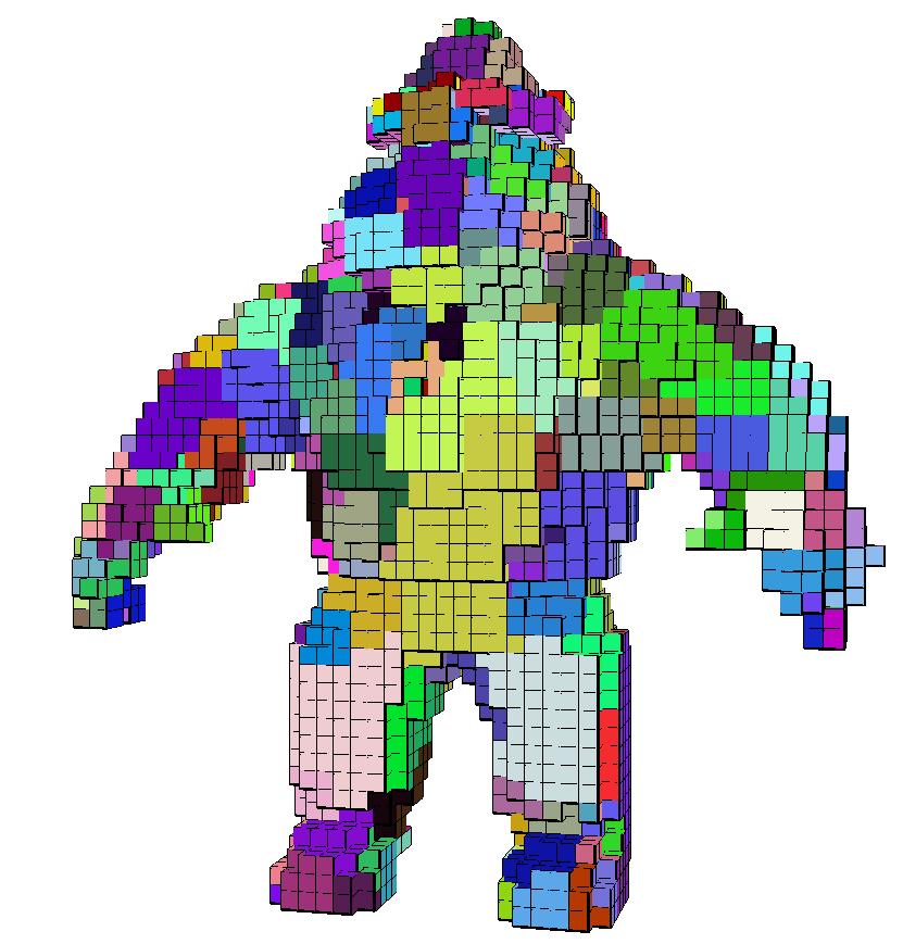
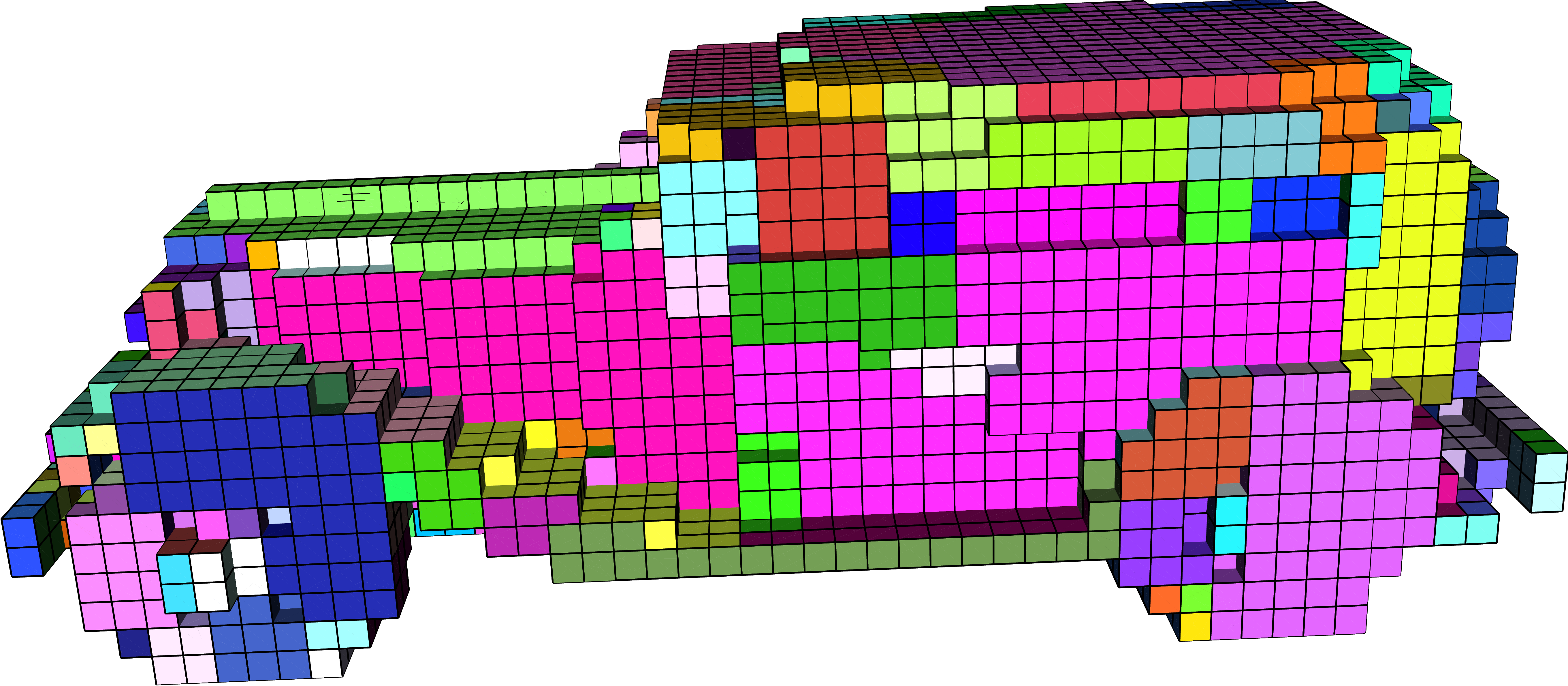
More difficult because of topological issues.
Idea: start from a topologically valid reversible triangulation (Marching Cubes), merge triangles using digital plane decomposition information and constraints on preimage


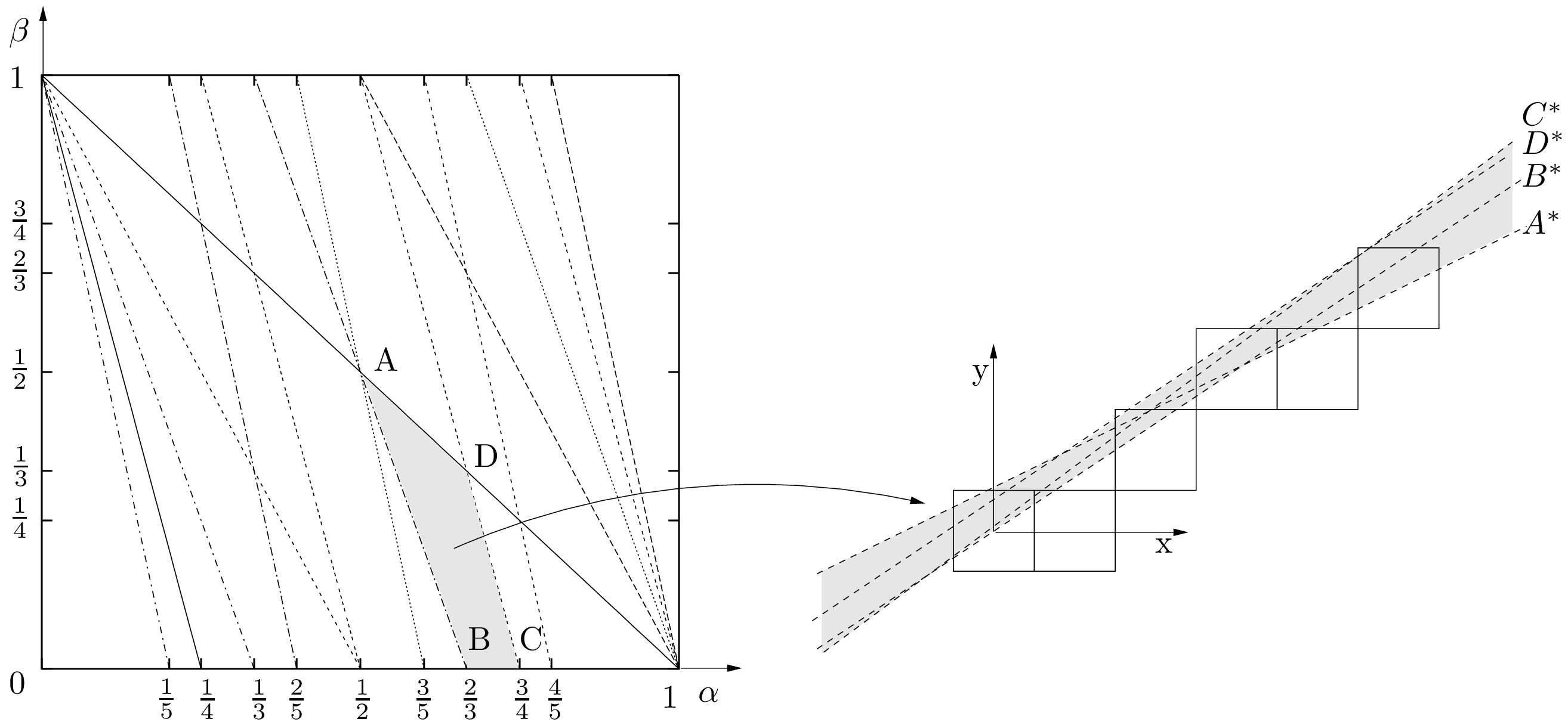
![\{(x,y)\,|\, y=\left [ \frac{-ax-\mu}{b} \right ] \}](_images/math/7ddb3453ec47f828c86a28172f311a250fb9964d.png)