Digital Geometry: Digital Model and Elementary Digital Topology§
| author: | David Coeurjolly |
|---|
| author: | David Coeurjolly |
|---|
Idea
Take benefit from the regular structure of the lattice to enhance geometrical analysis of shapes
|
|
|
Requirements
More formally
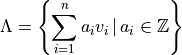
Lattice
Given a basis  of
of  ,
,
(finitely-generated free abelian group, symmetry group, …)
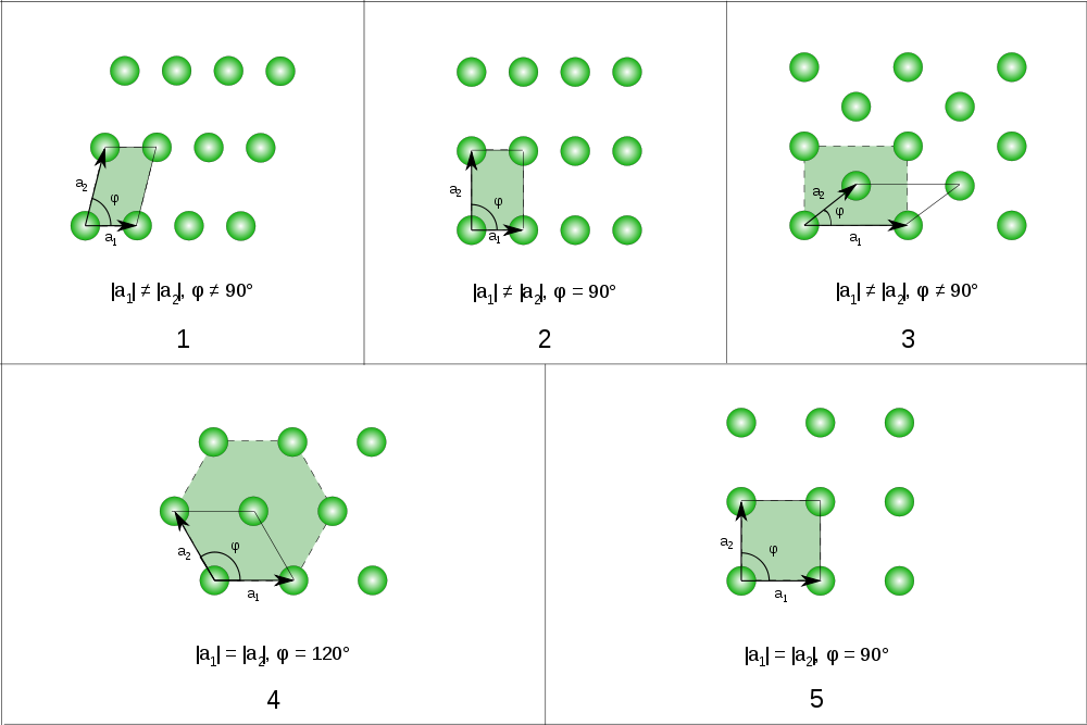
Five fundamental lattices in the Euclidean plane
 is its Voronoi cell
Following fundamental lattice classification: pavings by squares, hexagons, triangles, rhombi and parallelograms.
By definition, the paving induced by a lattice is periodic
Triangular/Hexagonal lattice/paving are dual
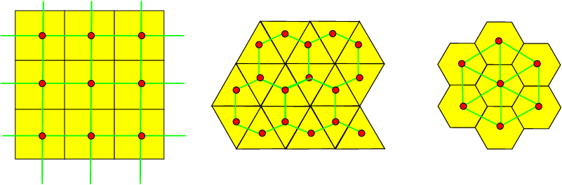
Speaking of density packing/kissing number and covering, hexagonal lattice is optimal
Regular cubic grid
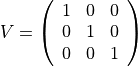
Face-centered cubic grid
Body-centered cubic grid
BCC has optimal covering
FCC has highest packing density and largest kissing number
FCC and BCC are dual
Hexagonal grid
Definition
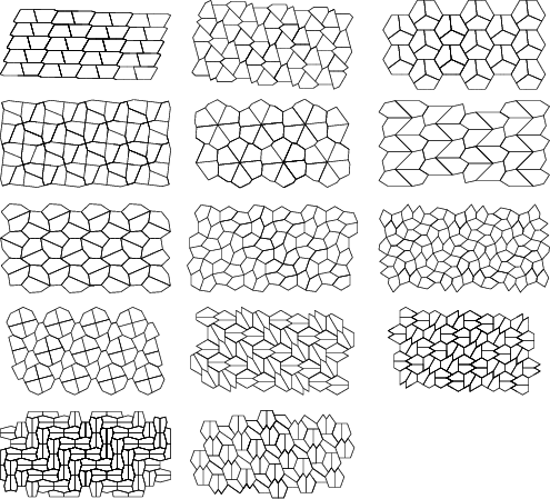
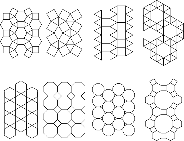
Several convex tiles paving the plane
No T-junctions
Same configuration of tiles around each vertex
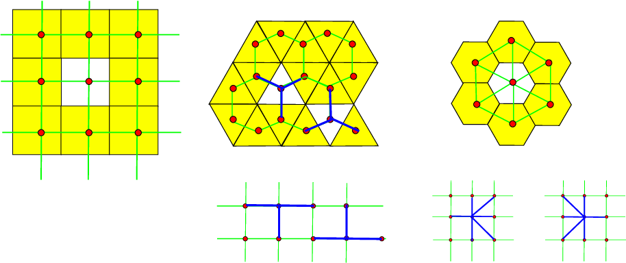
Square lattice
 , direct access to direct neighbors
  ,
, 
Triangular grid
, three direct neighbors (two local configurations when mapped to )Hexagonal grid
Lattice points: special encoding of lattice points to , six direct neighbors (two local configurations when mapped to )
Cubic grid
Trivial
FCC/BCC grid
Elongated grids
 Remapping
  on-the-fly
Combinatorial approach
In 2D:
and 
In 3D:
Topological approach
Two pixels/voxels are (k)-adjacent is the intersection of their (closed) cell is of dimension 
Mixing all dimensions:
 (1)-adjacent (0)-adjacent (2)-adjacent
(k)-path
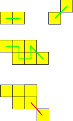
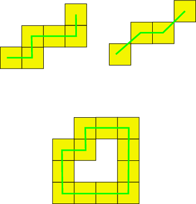
A sequence of digital points  is a (k)-path if for each point,
  is (k)-adjacent to
  (except for
  )
)
(k)-arc
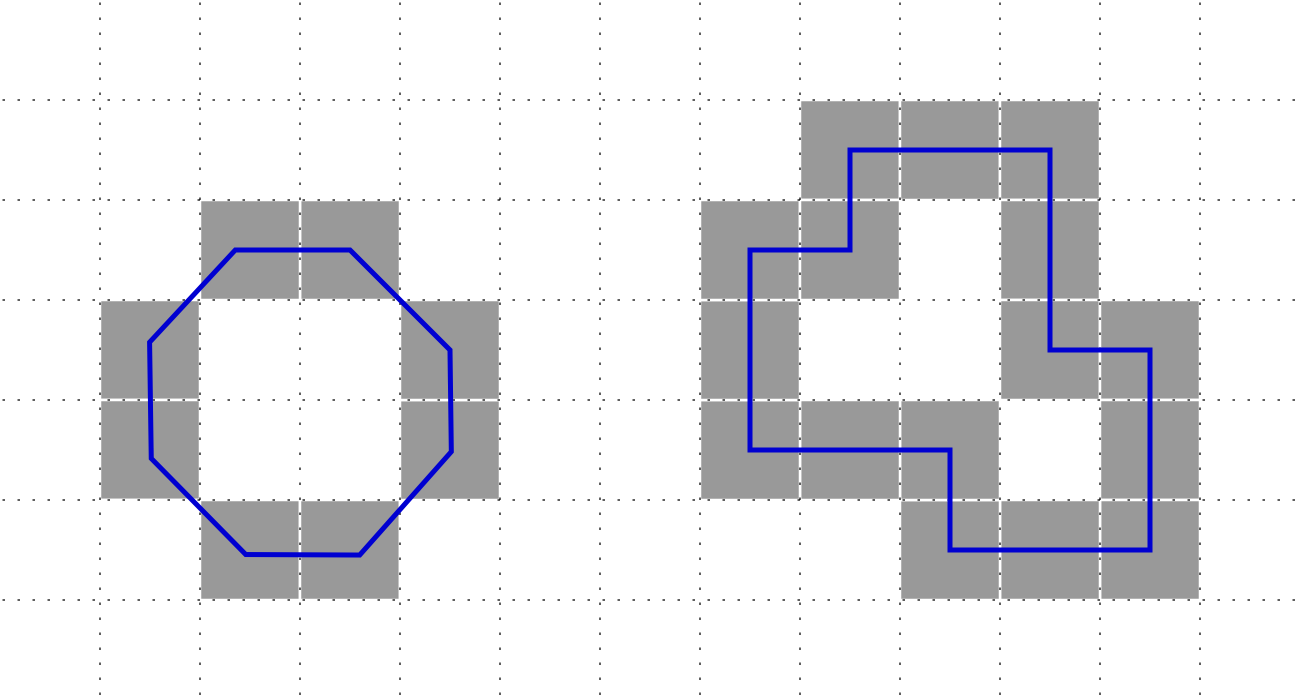
A (k)-arc is a (k)-path such that each has exactly two (k)-adjacent neighbors (except for extremities)
(k)-curve
A (k)-curve is a (k)-arc such that 
(k)-object
A set S of digital point is a (k)-object iff for any pair of points, there exists a (k)-path in S
|
|
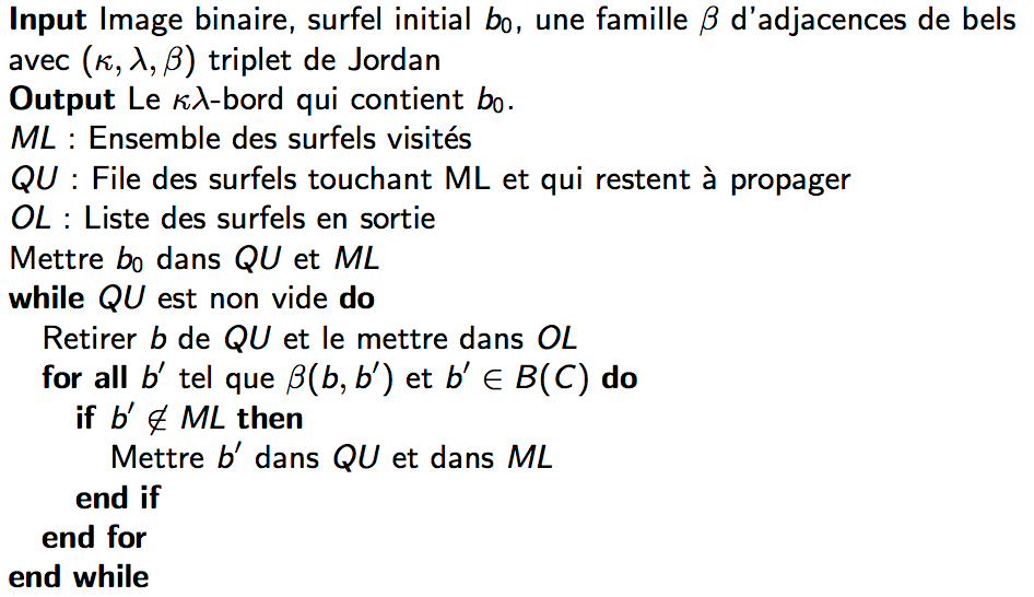
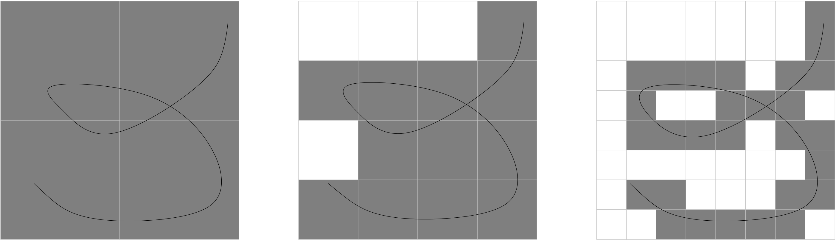
Can you spot (k)-arcs/(k)-objects/(k)-curves for  ?
?
Objective: define a notion of object contour/boundary matching with Jordan theory
 is a Jordan curve (or simple closed curve) in
  if is the image of a continuous and injective map from the circle to
 Jordan theorem states that:
 has two connected components, one is bounded (aka interior) and the other one is unbounded (exterior)
 from an interior point to an exterior one crosses (with an odd number of intersections)
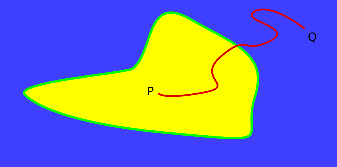
Idea mimic a digital version of Jordan framework replacing by a (k)-curve ?
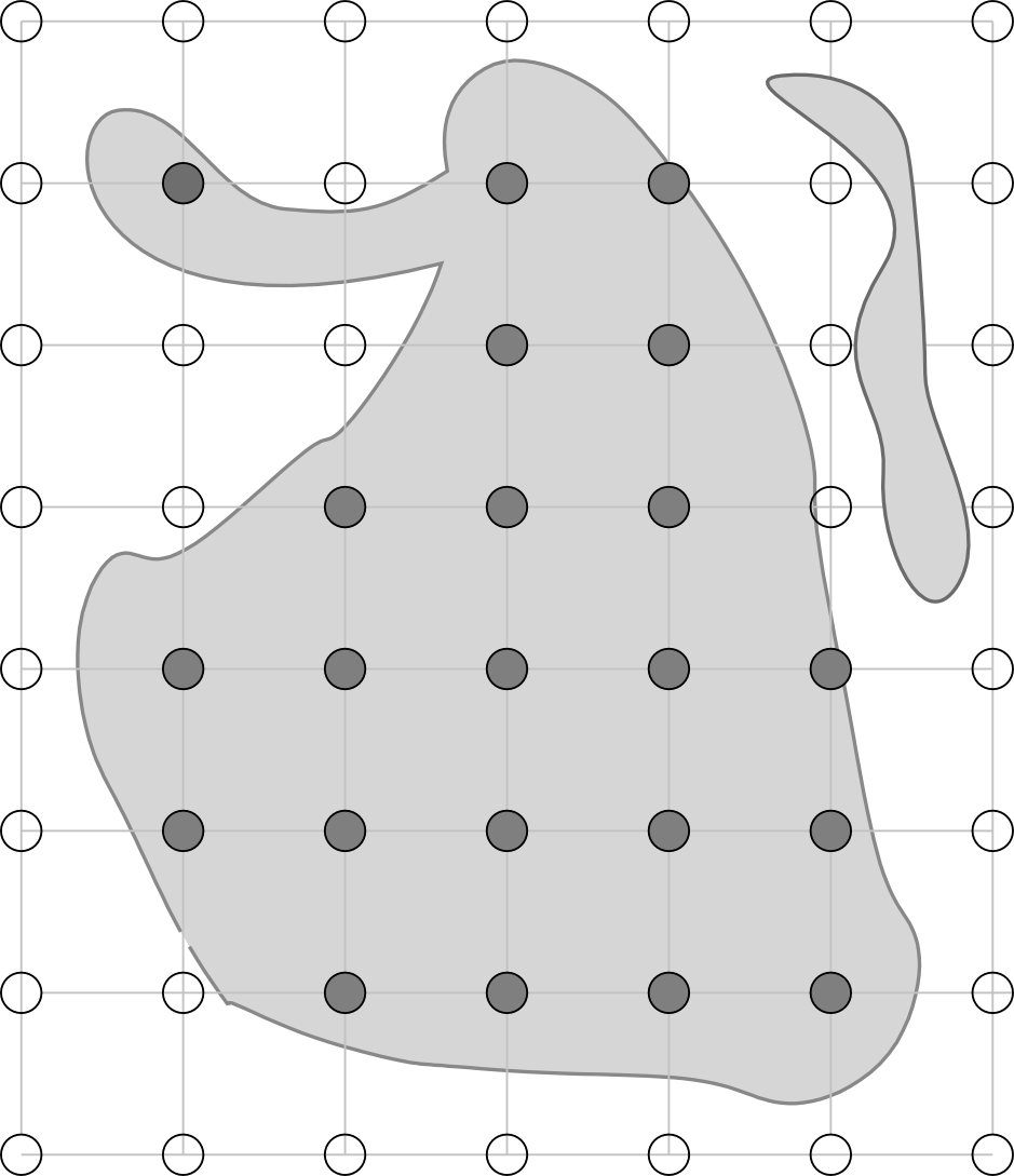
Given the following (0)- and (1)-curves, do they define Jordan-like curve ?
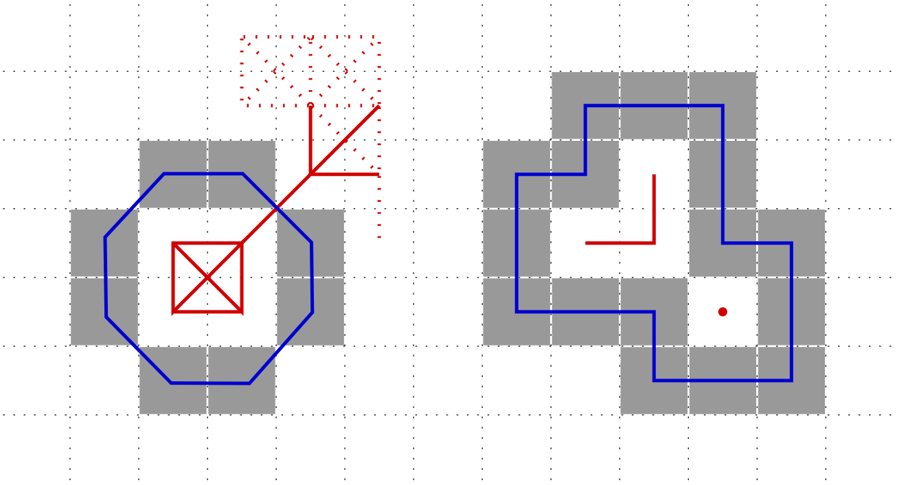
It depends…. we need a pair of adjacency relationships !
 Jordan pair such that k is the adjacency for the object and l the adjacency for the complementary
In dimension 2
(0,1) and (1,0)
In dimension 3
(2,1), (2,0) (1,2) and (0,2)
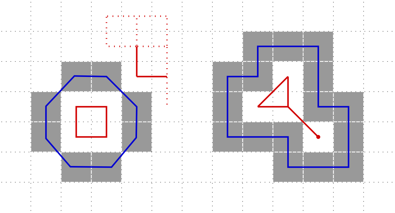
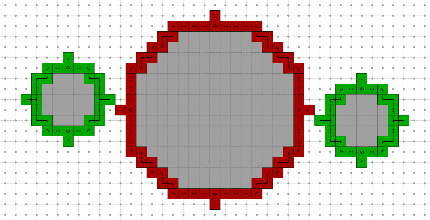
Border: Given a Jordan pair, the border of  is the set of
  -adjacent digital points which are
  -adjacent to points in
-object but we need more constraints to have a -curve (or kind of, both are considered as open sets)
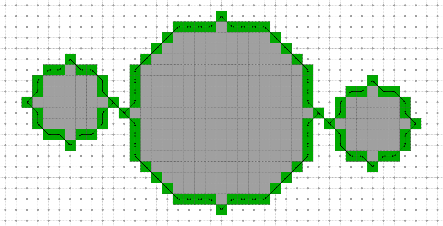
|
|
Idea embed the digital space  into a cellular space (cartesian cubic space) to represent oriented inter-pixel elements
In 2D
are embedded into 0-cellsIn nD
(two 0-cells, two 2-cells and four 1-cells)
Principle defines digital surface as a set of (n-1)-cells (surfels)
 relationship on surfels (anti-reflexive, local transitive closure, locally defined) Jordan adjacency pair,
  triplet is a Jordan triplet
We can demonstrate that such Jordan triplets leads to well-defined digital Jordan surface
Illustration in 2D (here, k=1)
Approach is valid for various digital structures
in 3D§Two valid relationships on (2,1)- or (2,0)- pairs on closed objects
relationship + graph traversal (depth first, breadth first,…) digital surface tracker
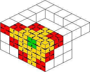
|
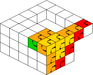
|
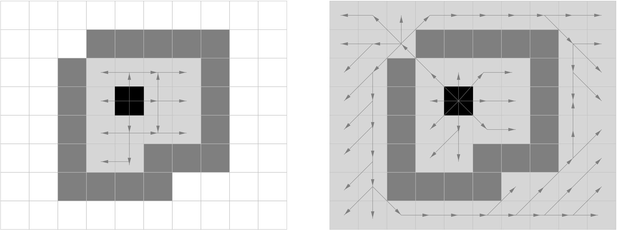
Efficiency of the tracker is guided by the `beta`:math: complexity
For (2)-object
is not oriented, each surfel is processed 4 times with oriented arcs (2 arcs per surfel), each surfel is processed 2 times
 with oriented arcs (1 or 2 arcs per surfels), each surfel is processed 4/3 times (on average) Hamiltonian path exists if is homeomorphic to a ball
Overall algorithm (for single connected surface)
Complex Objects
Several connected components, holes, …
Scan the complete volume, mark all surfels as potential starting surfels and apply the tracker on each starting surfel (removing traversed surfels)
Formalize the embedding 
- Jordan for some grid steps)Let  and its digitization
 0 but even in this case, may be empty
 to ensure topological properties on or
This model was first used to approximate
by
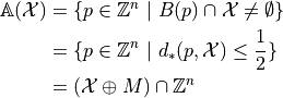
Idea Defined for oriented contours 
For each intersection with a grid edge, we select the {closer,inner,outer} grid point
(resp. GIQ -Grid Intersect Quantization-, OBQ -Object Boundary Quantization-, BBQ -Background Boundary Quantization-)
crosses the edge at its mid-point) global Oracle to remove ties and Generic definition
Let  be a metric,
  its unit ball and
Still bubbles may exist
Following the definition (F,G  ):
):
prop.


Allows modeling of digital objects but CSG approach (Constructive Solid Geometry)
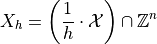
Idea Digitization parametrized by a grid step
E.g. for Gauss digitization
Mathematical results can be obtained with constraints on , for example
thm.
If  is
is  with bounded curvature, there exists a grid step
  such that for
  ,
,  is topologically equivalent to
thm.
If is with bounded curvature, the retro-projection from  onto at
  along its normal direction is continuous, mono-valuated and surjective (for ) and
  )
)
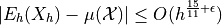
Question 1 Given a digital object, How to estimate its areas ?
Answer Well, let’s count the number of grid points (unit squares) (estimator denoted E)
Question 2 Is this estimator multigrid convergent ? What is the convergence speed ?
Answer
Let’s consider the estimator  at grid-step h defined on the digitization of the Euclidean shape from a given class of shapes
If is a finite convex shape, there exists a grid step such that for we have:
[Gauss, Dirichlet]
If is  (or finitely piece-wise with positive curvature almost everywhere…) then
[Huxley,…]
Would there be better approaches ?