Digital Geometry: Volumetric Analysis§
| author: | David Coeurjolly |
|---|
| author: | David Coeurjolly |
|---|
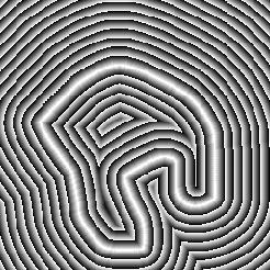
Distance transformation
Def.
At each point  of a shape
  , we want the smallest distance to
|
|
|
 We need

Very usefull
…for many applications
|
|
|
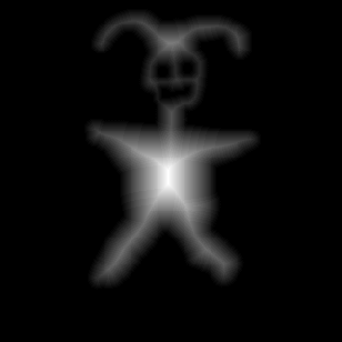
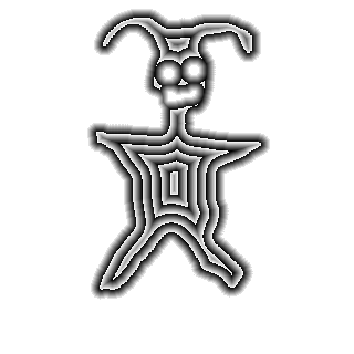
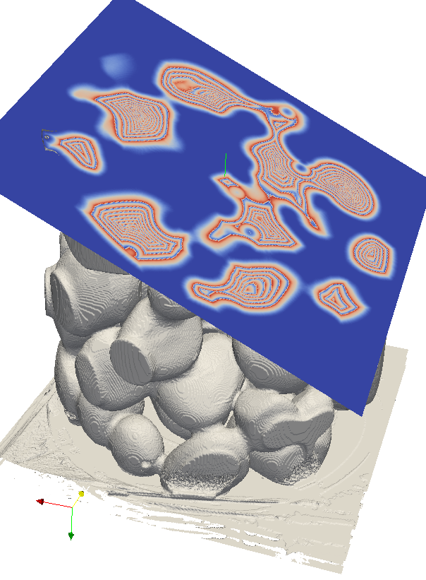
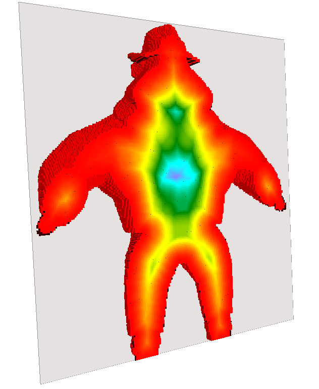
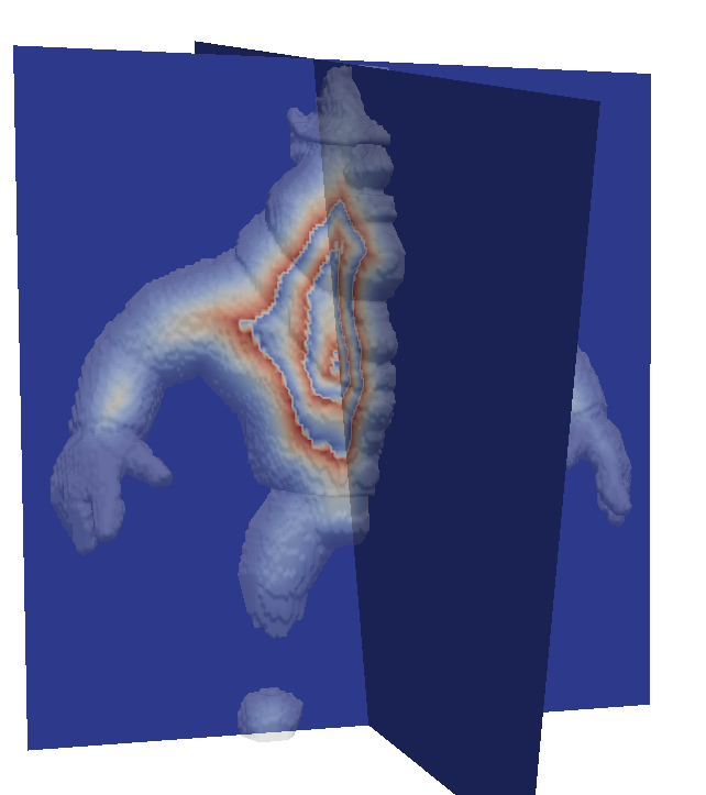
Idea
Shape  Boundary Distance field Implicit representation
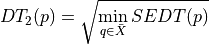
Objectives
DT)
|
|
|
Objectives
DT)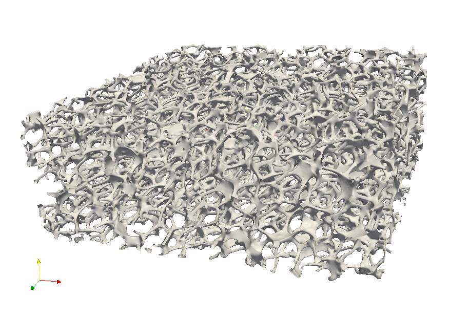
|
|
Def.
Metric  is a map
  such that
 (separation axiom)
 (coincidence axiom)
 (symmetry)
 (triangular inequality)
Def.
is a norm (metric induced by “normed” vector space) iff
 (translation invariant)
 (homogeneity)
E.g.


 metric:
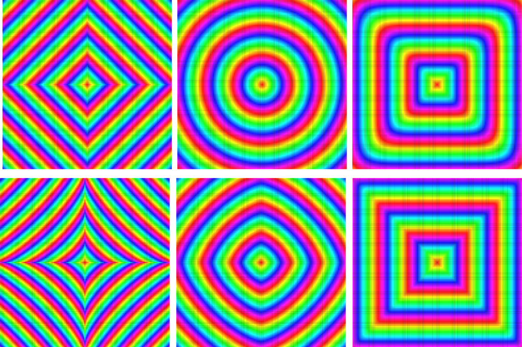
Definition

Hence
 ,
,  are Discrete Metrics
 is not a discrete metric
 is not a metric
 is a discrete metric
 is a not discrete metric
![[d_2]](_images/math/cead7f2a8fdc71f0fdcf6aad89394bc45b4a1fb4.png) is not a metric
is not a metricHints for last two results use 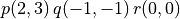 and
and 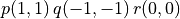
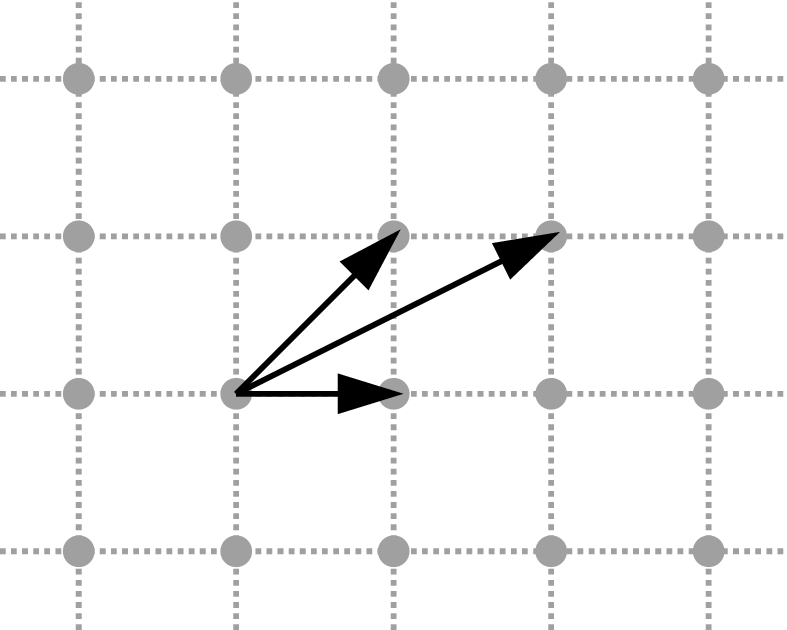
Weigthed vector
Chamfer Mask
Set of weighted vector
Usually, chamfer masks are G-symmetric, i.e. restricted to
with
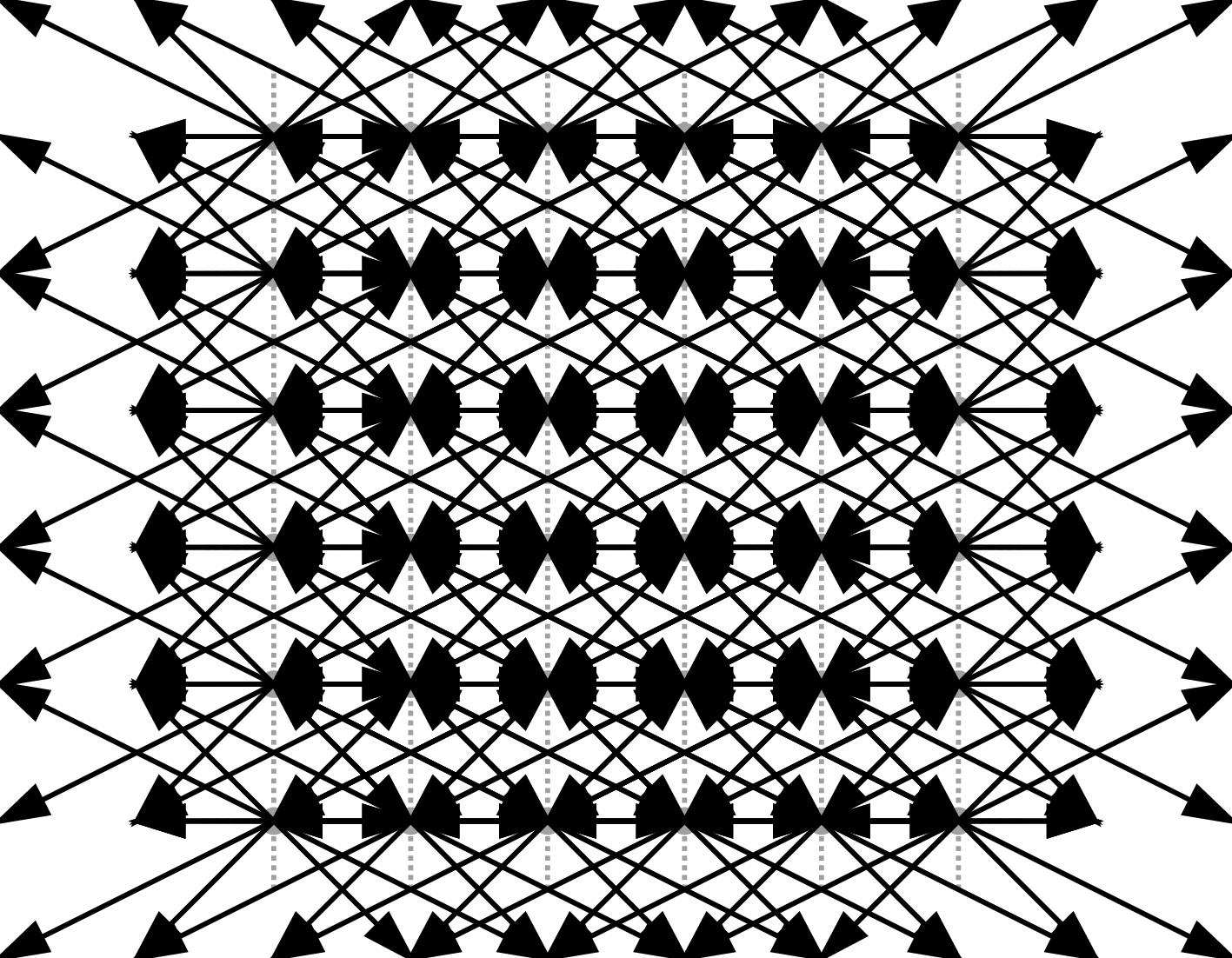
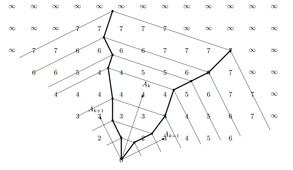
Chamfer path
 -Path based on vectors from a chamfer mask
Length of a chamfer path
Chamfer distance
Minimal length of chamfer path between
and

All chamfer distances induced distances, not necessarily norm
Path based distance
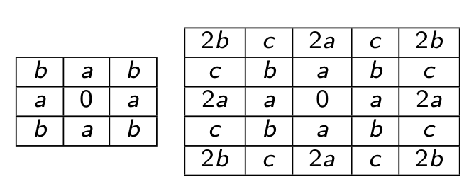
Matrix representation for masks
 ,
, 
For example:
(distances must be divided by 3 at the end)
We need constraints on  to induce norms
e.g.
We construct the mask to approximate the Euclidean Metric
 ) on specific configuration

Drawbacks
Propagation using Dijkstra’s algorithm
vertices and edges taken from 
Computation cost in  for
for  grid points and
|
|
|
Split the mask into two sub-masks and perform forward/backward scans with “min” operations.

Computational cost in 
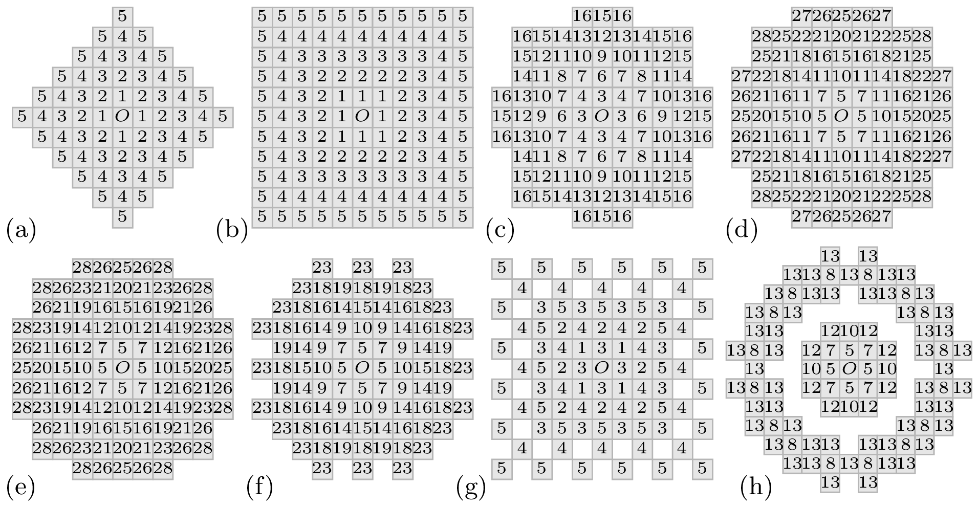
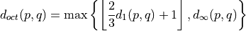
Neighborhood sequence


Example
“Octogonal” distance with infinite sequence 
Sometimes, explicit forms exist
Idea
Still consider  distances but with integer based representations and algorithmic
E.g.
 by
by  by vector
 by
by  or even for metrics
Nice but are there fast algorithms for such exact metrics ?
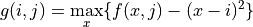
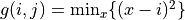
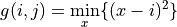
We want to compute (for all  )
)
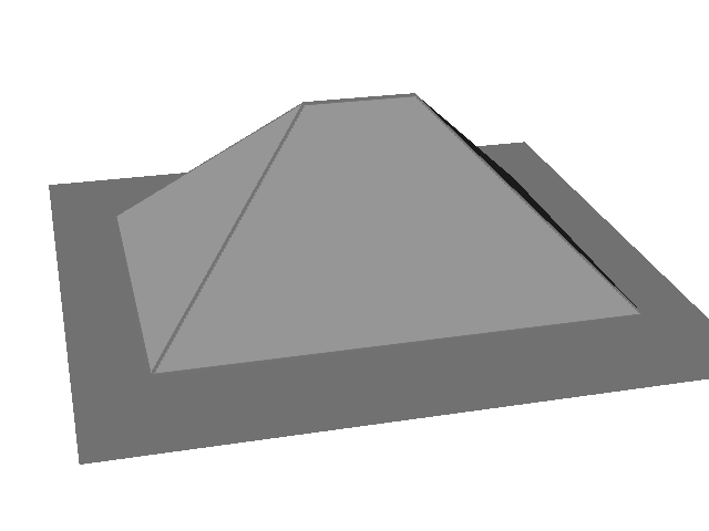
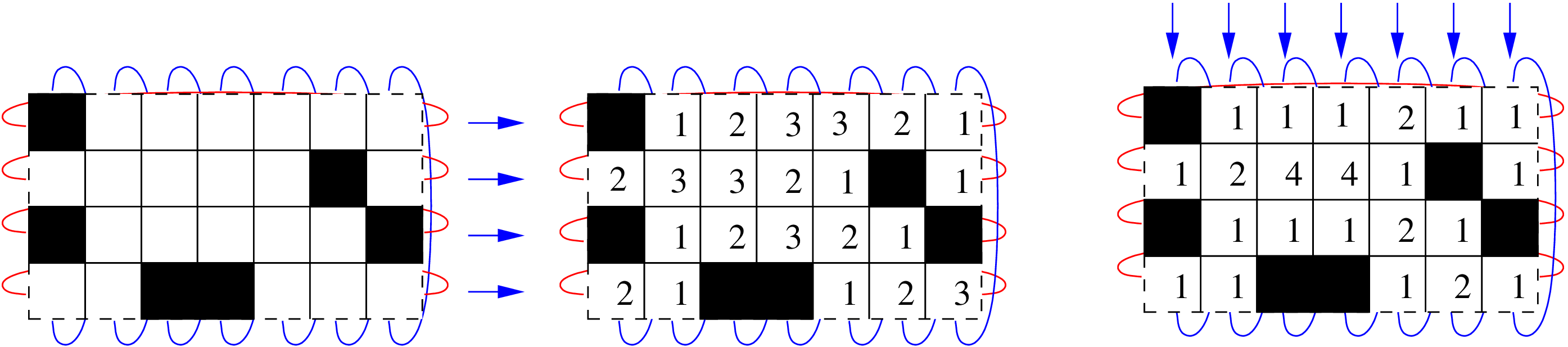
Separable approach with intermediate map
in dimension 3, we would have
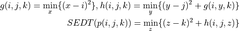
Simple two-scan propagation
 in 2D for NxN image
 in d-D for N^d image
 and
and 
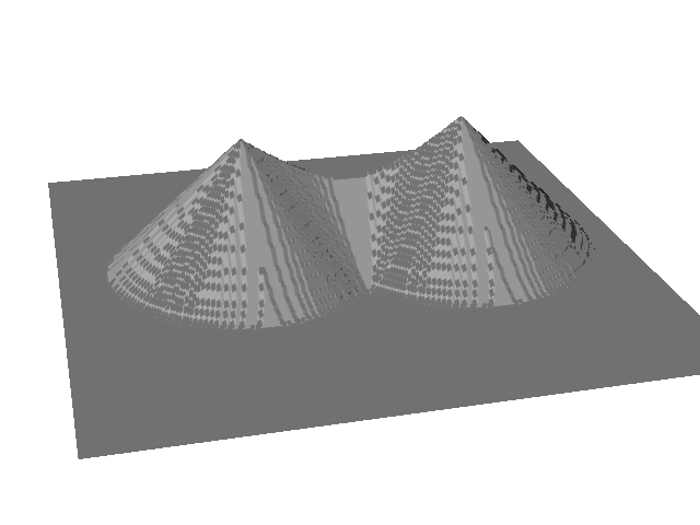
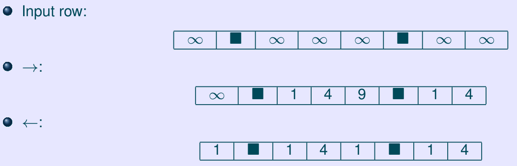
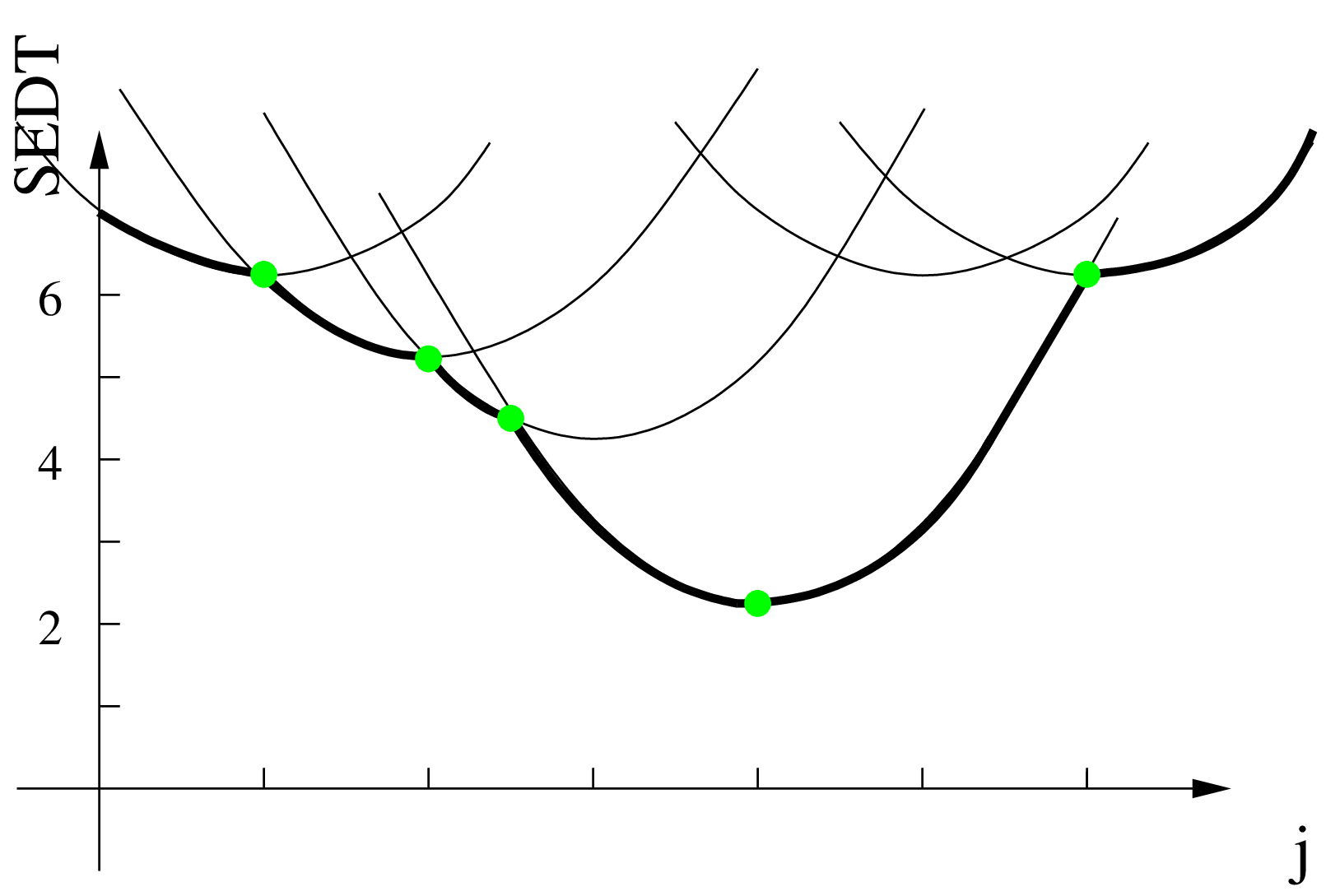
Key-point Lower envelope computation of a set of parabolas
Consider the set of parabolas 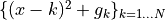
 and
and  are two parabolas with intersection and
  cannot appear in the lower envelope for abscissa greater than
 Lower envelope computation in  using stack based approach ;)
Given a  image
image
Algorithm
 remaining dimensions: compute independent lower envelope which are in
  algorithm for error free Euclidean metric DT
|
|
Thanks to separability
Optimal multi-thread implementation
Generalization to toric domains
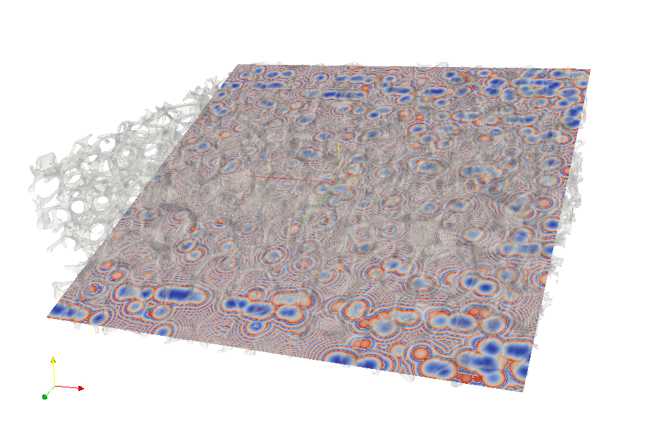
Useful to characterize periodic structures in arbitrary dimensions
Principle
Def.
We consider  ,
,  with
with 
 be a point on the x-axis such that
Let  be another point on the x-axis
A metric
be another point on the x-axis
A metric  is monotonic if
Result
metrics are monotonic Let’s use the separable approach for other metrics !
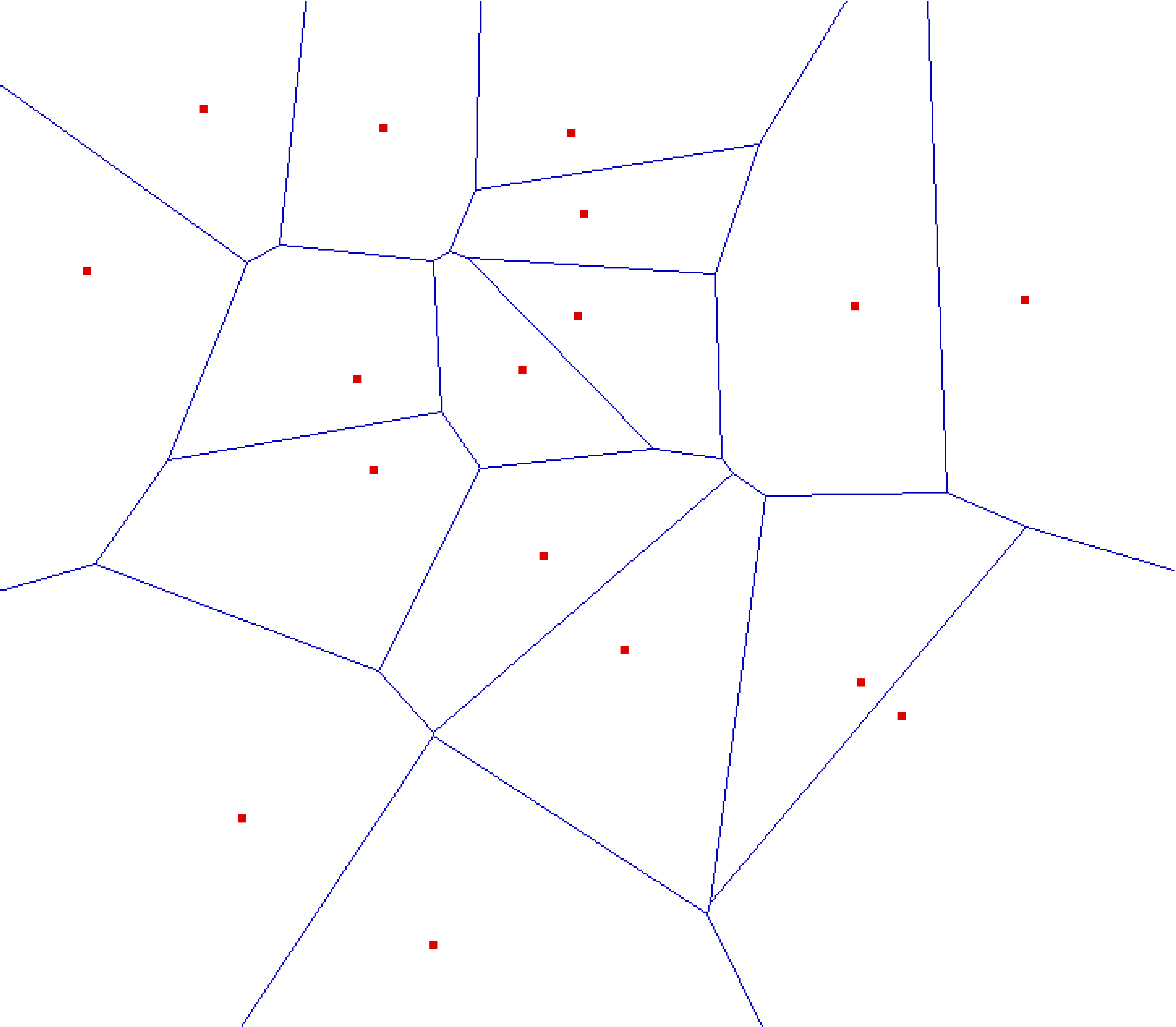
Definition
 , the Voronoi Diagram is a decomposition of the space into closed cells
  such that
Each cell can be further decomposed into sub-dimensional i-facets taking into account cases where 
Voronoi Diagram  Distance Transformation
Getting the distance value is equivalent to localizing a point in a Voronoi diagram
Input set:  , we construct

|

|

|

|

|

|
Main Result
For any monotonic metric and an image ![[1\ldots n]^d\rightarrow \{0,1\}](_images/math/1320afc9a136676702fdf76c54f4309d526ff1b7.png) , the Voronoi Map (and the distance transformation) can be obtained by the separable algorithm in , the Voronoi Map (and the distance transformation) can be obtained by the separable algorithm in  |
|
|
| Metric | C | H | Total |
|---|---|---|---|
 |
 |
|
 |
 |
|
|
|
 |
|
|
|
| Exact |
 |
 |
 |
| Chamfer Norms |  |
 |
 |
| Neigh. Seq. Norms | O(1) |  |
 |
Better expected bounds for path based norms
| Metric | C | H | Total |
|---|---|---|---|
| Chamfer with adapter |  |
 |
 |
| Chamfer Norms |  |
 |
|
Similar expected results for neighborhood sequences
Notations
Chamfer masks:  (we consider only chamfer masks inducing norms)
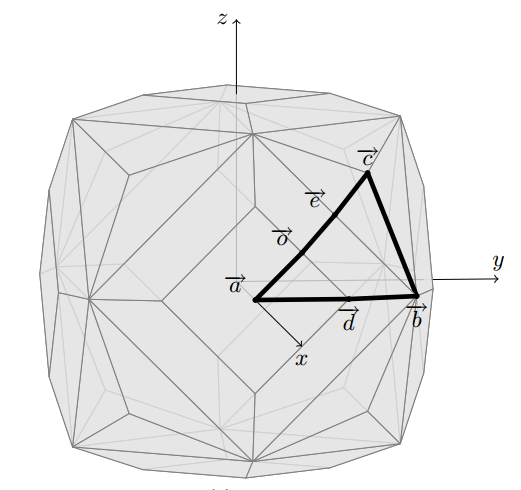
Rational ball:  [Normand, Strand,…]
Rational ball faces have normal vector 

[Normand et al.]
Can be generalized to other path based distances to get similar expression
for some function  (based Lambek-Moser inverse sequences)
Computational Geometry setting
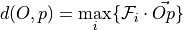
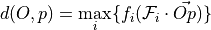
 is given by the facet pierced by the straight line
  Ray shooting problem in convex polytopes
Fast Distance computation
Following [Matousek and Schwarzkpof]
 space/pre-processing and
 per query
Goal
 then we have exact Voronoi Map/DT in

Main Result
==> First sub-quadratic DT algorithm for Chamfer metrics
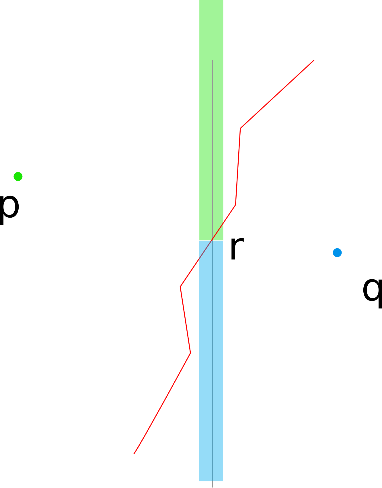
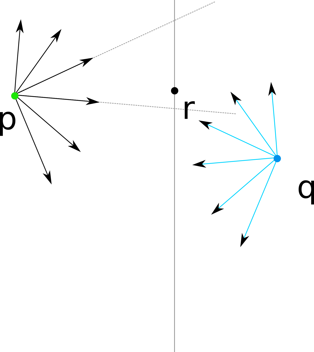
Key point
Given to points and a straight line, detect the position of the Voronoi edge on the line
we are looking for point  such that
Question Find the cone at containing a point 
==> Dichotomic/Binary search (thanks to convexity of the metric)
==>
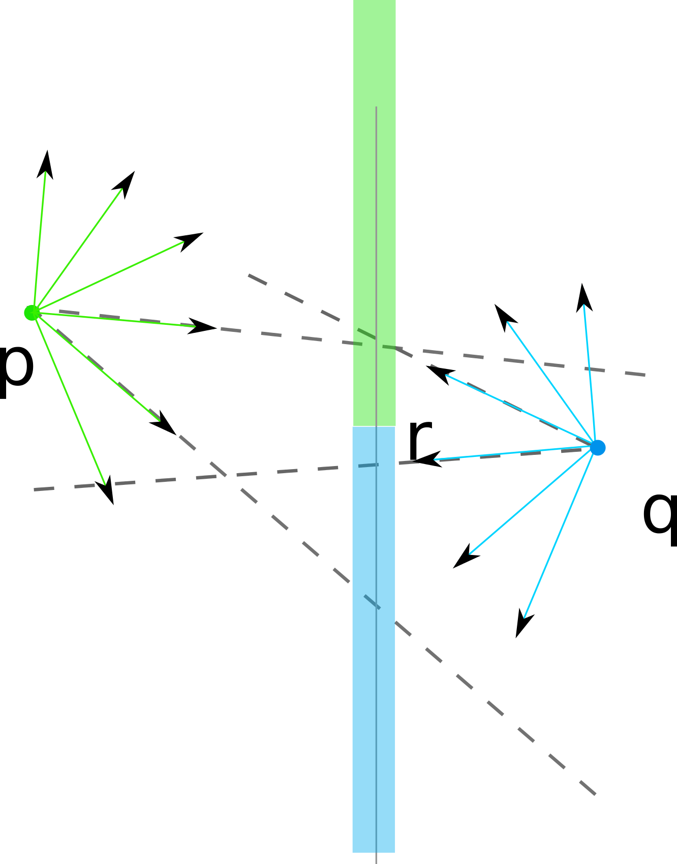
Idea
If we have localized the Voronoi edge point, we are done (find the exact position given by linear system with one unknown)
 §
§ShrinkMp( Mp, Mq )
if |Mp| == 1
return the cone in Mp
else
Split cones Mp -> { Mp, cone, M-} with |M+|~|M-|
{v1,v2} = cone
dp1 = distance d_M(p, v1 intersection l) //O(1)
dp2 = distance d_M(p, v1 intersection l) //O(1)
dq1 = localize and get the distance of d_M(q, v1 intersection l) //O(log(m))
dq2 = localize and get the distance of d_M(q, v2 intersection l) //O(log(m))
c1 = closest point between p and q at v1
c2 = closest point between p and q at v2
if (c1 == c2 == GREEN)
return ShrinkMp(M+)
if (c1 == c2 == BLUE)
return ShrinkMp(M-)
return cone
Correctness
 and final computation§
Shrinking
cone
Final step

Basic Idea for in 

 defines a plane (
 )
) induces a 2-dimensional polytope 2D problem with
  computational cost
Conclusion
Closest() and HiddenBy() predicates can be implemented in 
Exact Voronoi map/Distance transformation of Chamfer norms using separable approach in
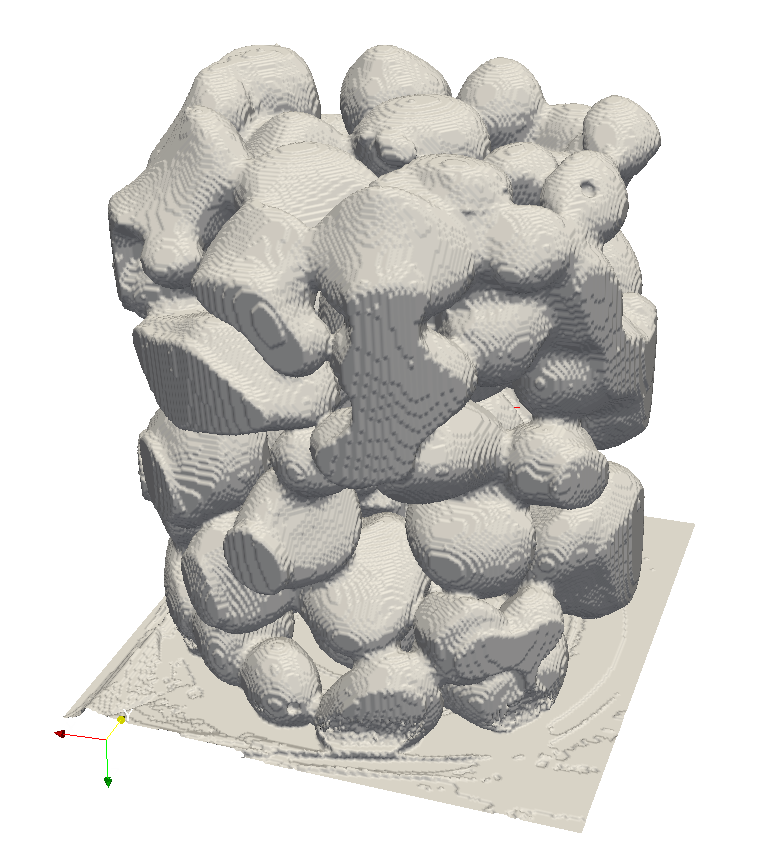
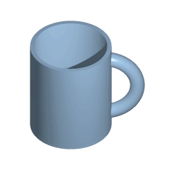
Problem setting
Def.
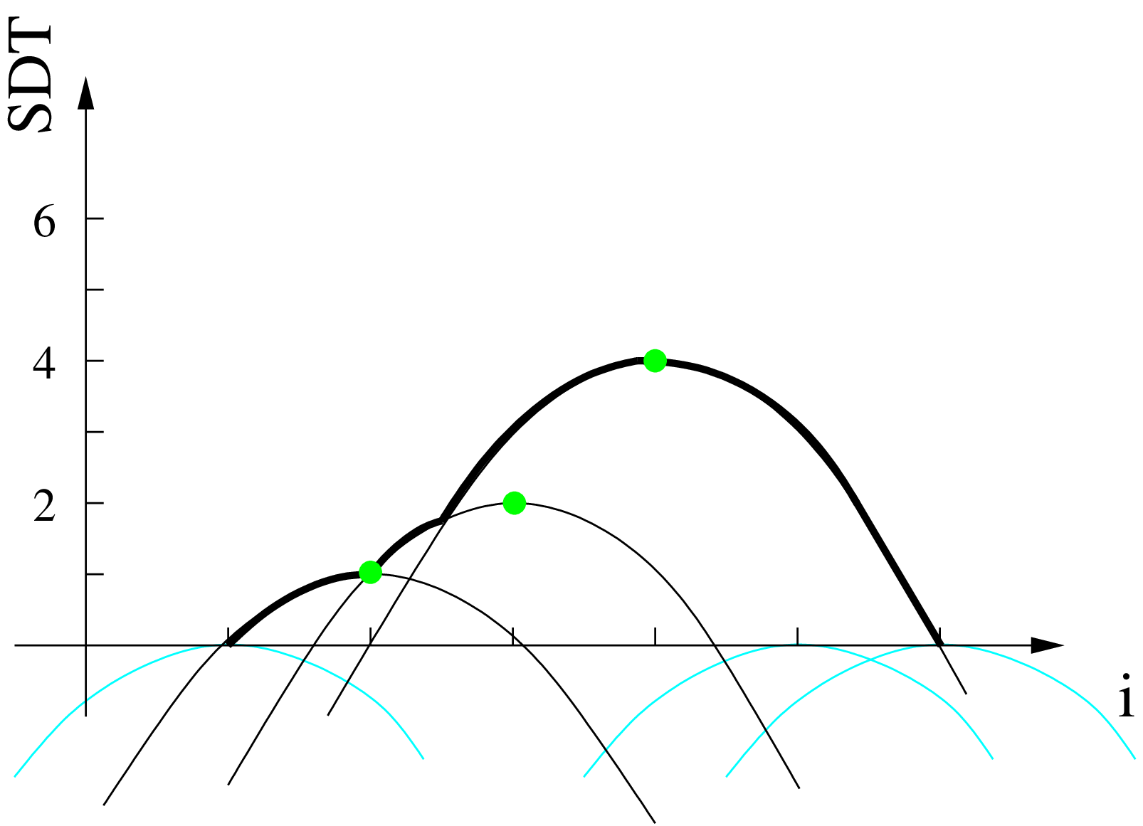
Given a metric  and a set of balls
  , reconstruct the binary shape
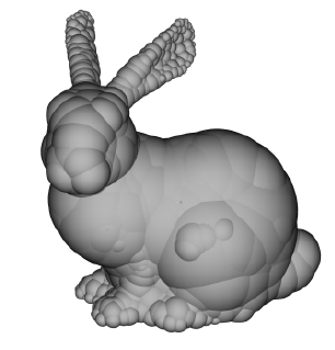
Why?
Reverse operation of the Distance Transformation
To reconstruct the shape if we characterize it as a union of balls (e.g. via medial axis)
Bruteforce approach
For  image
image
§W.l.o.g. we consider 
Let us denote  for
for  , then
Which can be rewritten
Separable decomposition
Start from a map  with
with  if
if 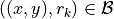 (
( otherwise)
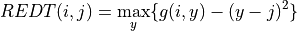
Similar algorithm
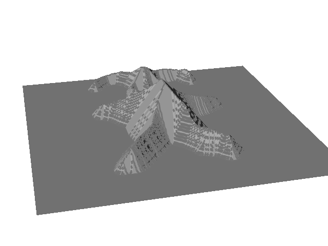
Upper envelope computation of a set of parabolas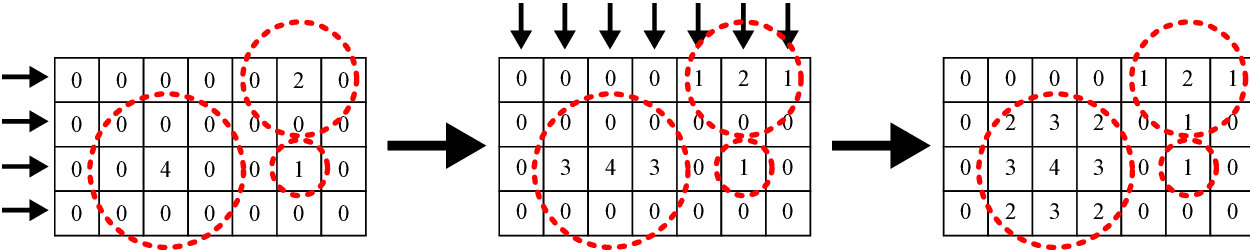
 separable algorithm for REDT
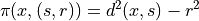
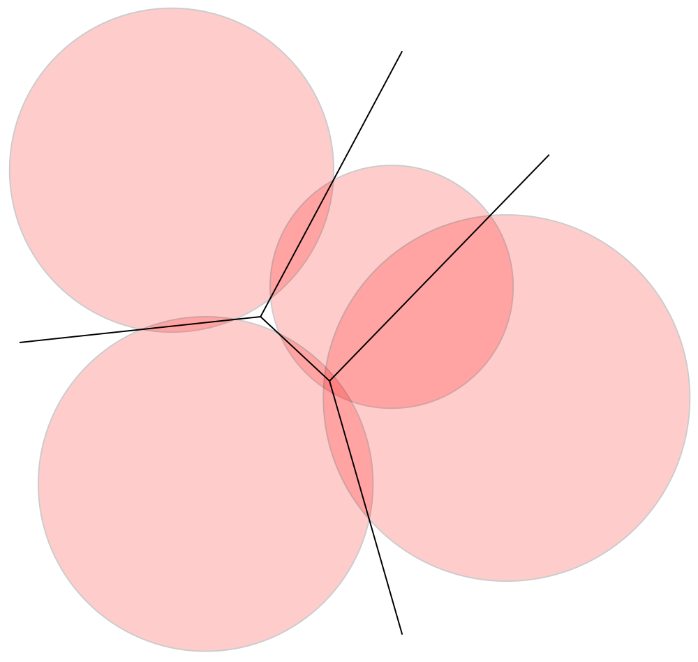
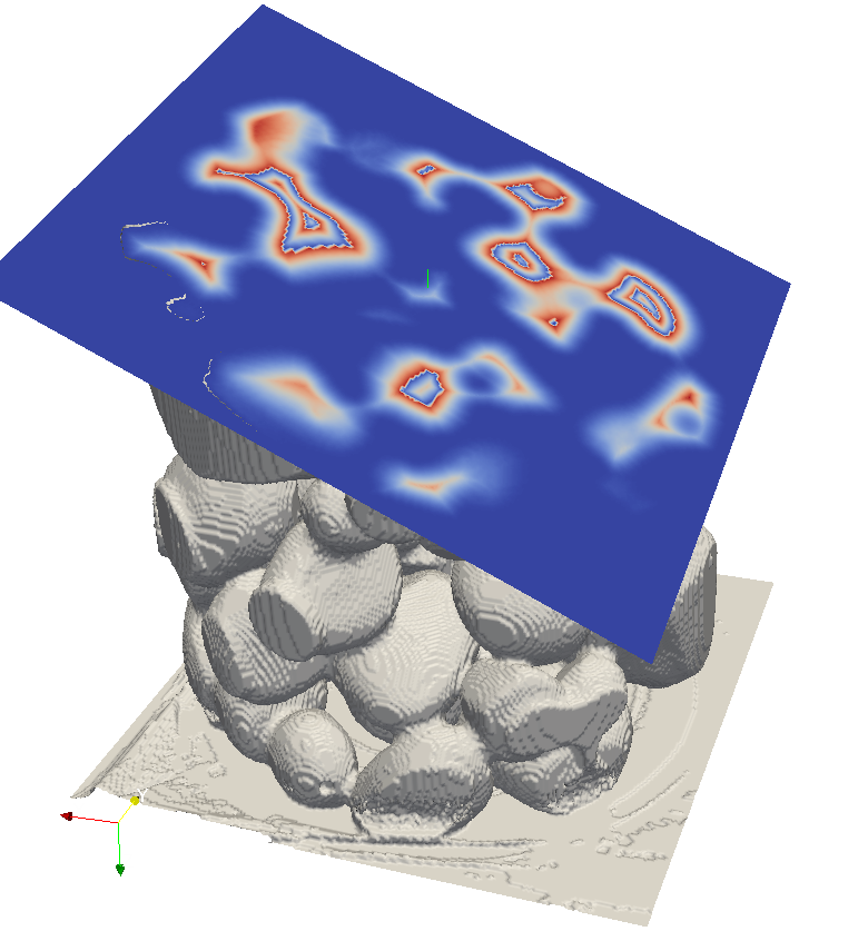
Voronoi map –> Power map
Kind of Voronoi diagram with additive power metric. For example the power of a point x w.r.t. ball 
Def.
 , the Power Diagram is a decomposition of the space into closed cells such that
Each cell can be further decomposed into sub-dimensional i-facets taking into account cases where
|

|
Idea
 is equivalent to the construction of
Results
computational cost for a large class of metricsAlternative Definitions
PDE fromulation) is maximal in X if
 at least twice
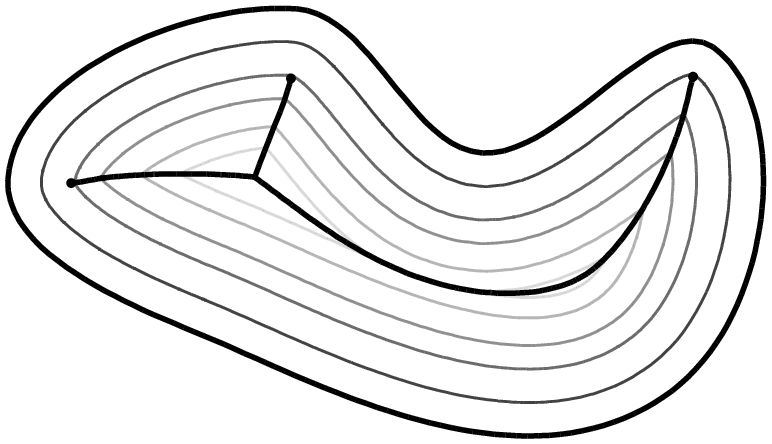
|
|
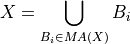
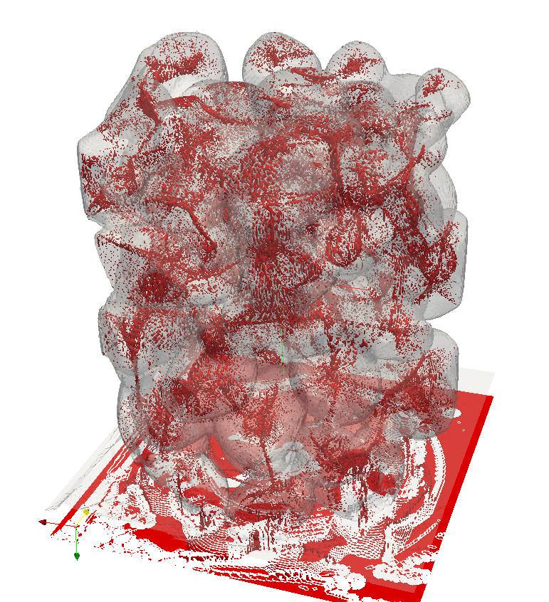
Voronoi Based Approximation
Shape
Point set approximation
Voronoi Diagram
Medial Axis approximation
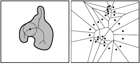
Convergence results exists for various classes of Voronoi based medial axis
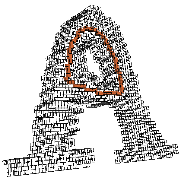
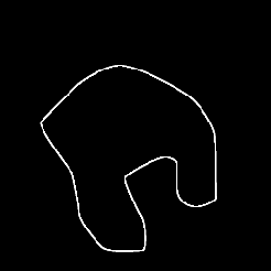
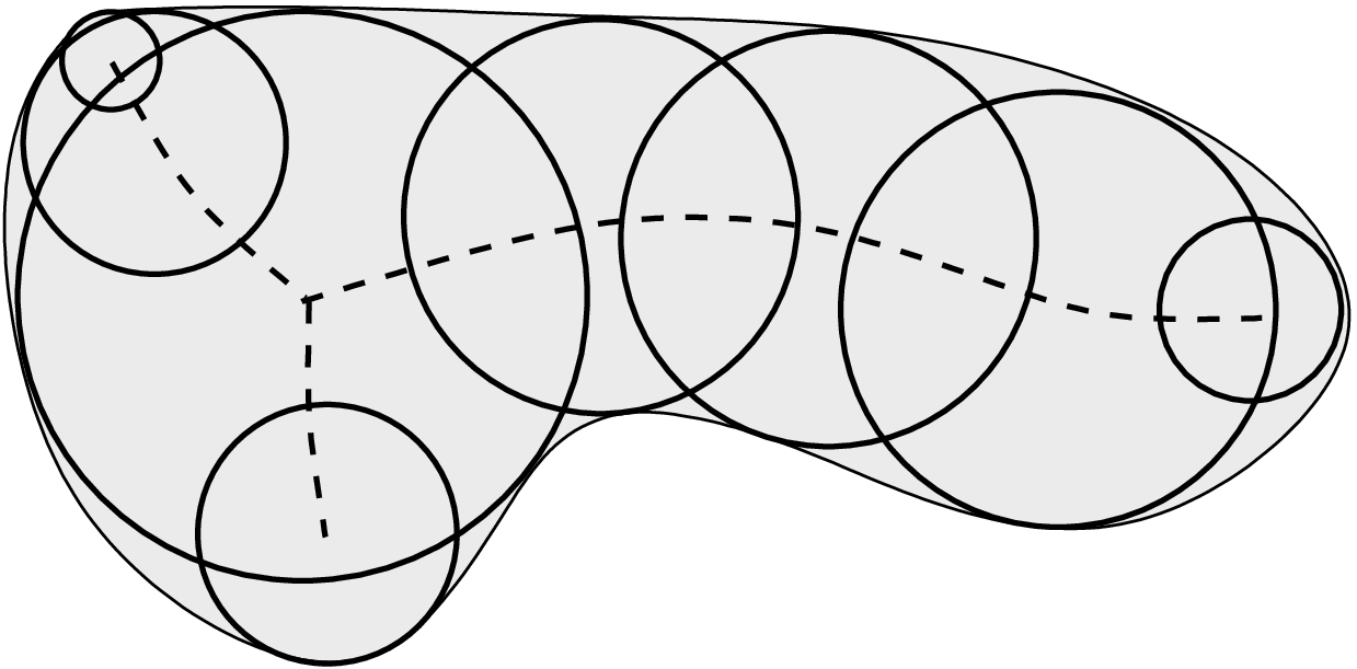
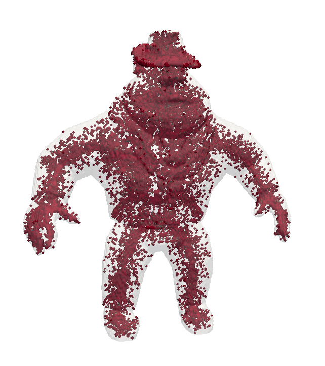
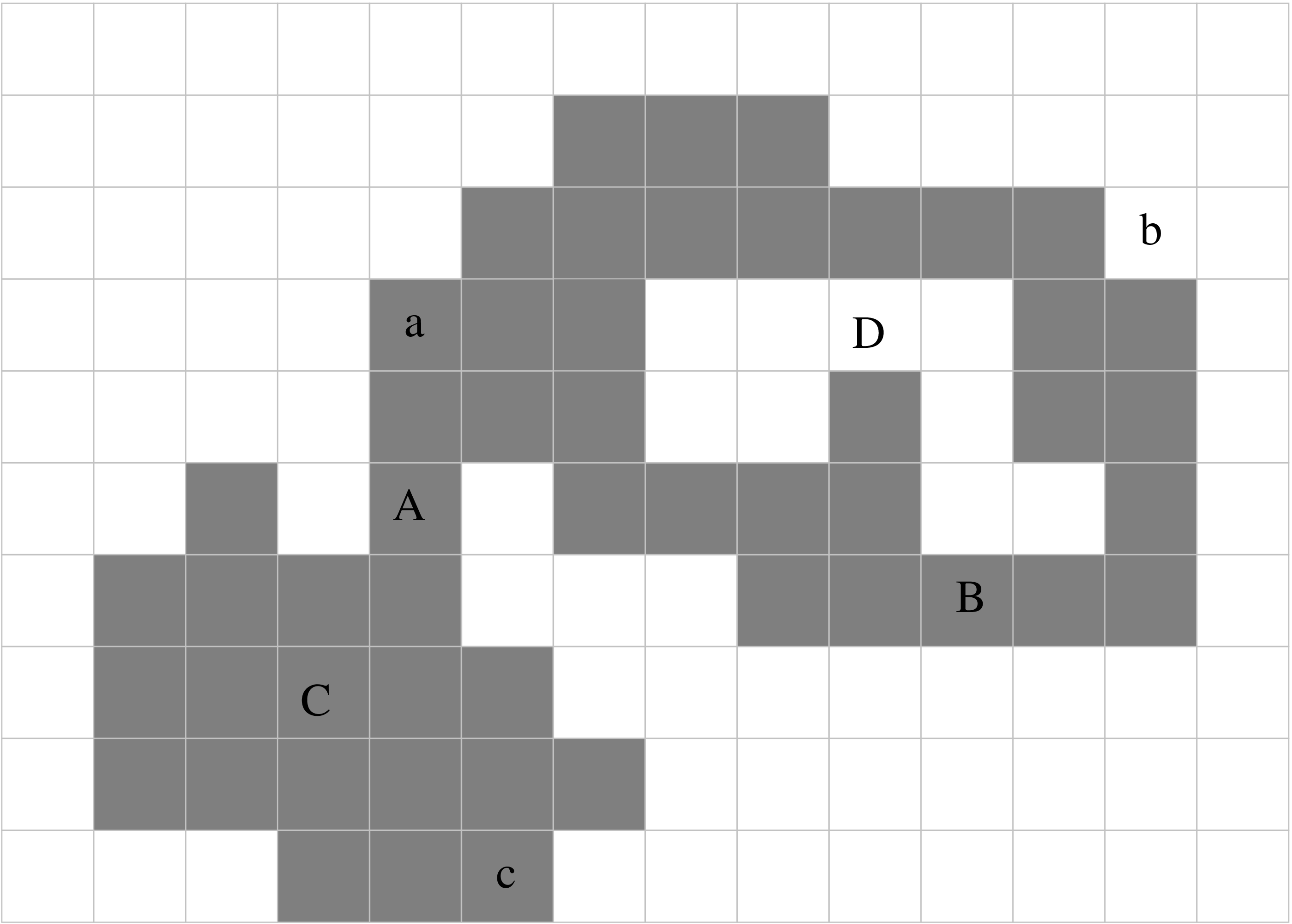
Def.
A maximal ball is a ball contained in the shape not entirely covered by another ball contained in the shape
Def.
The medial axis of a shape is the set of maximal ball centers contained in the shape.
Digital Setting

 Finite set of digital balls contained in Medial Axis Extraction Combinatorial Covering problem
Reversible Encoding of X
DT as preliminary step
Given and  such that Euclidean ball with
  , we have
(defined for but trivial generalizations to other metrics)
|
|
|
Set of candidate balls 
Covering Test
Let us consider a IsCoveredBy(B,B’) a predicate returning true if 
If B and B’ are Euclidean balls The predicate is in
If B and B’ are Digital balls The predicate is in 
but

Bruteforce Digital Medial Axis Extraction  (with
(with  the maximal DT value)
Goal
Design a IsCoveredBy() predicate with cost as a function of 
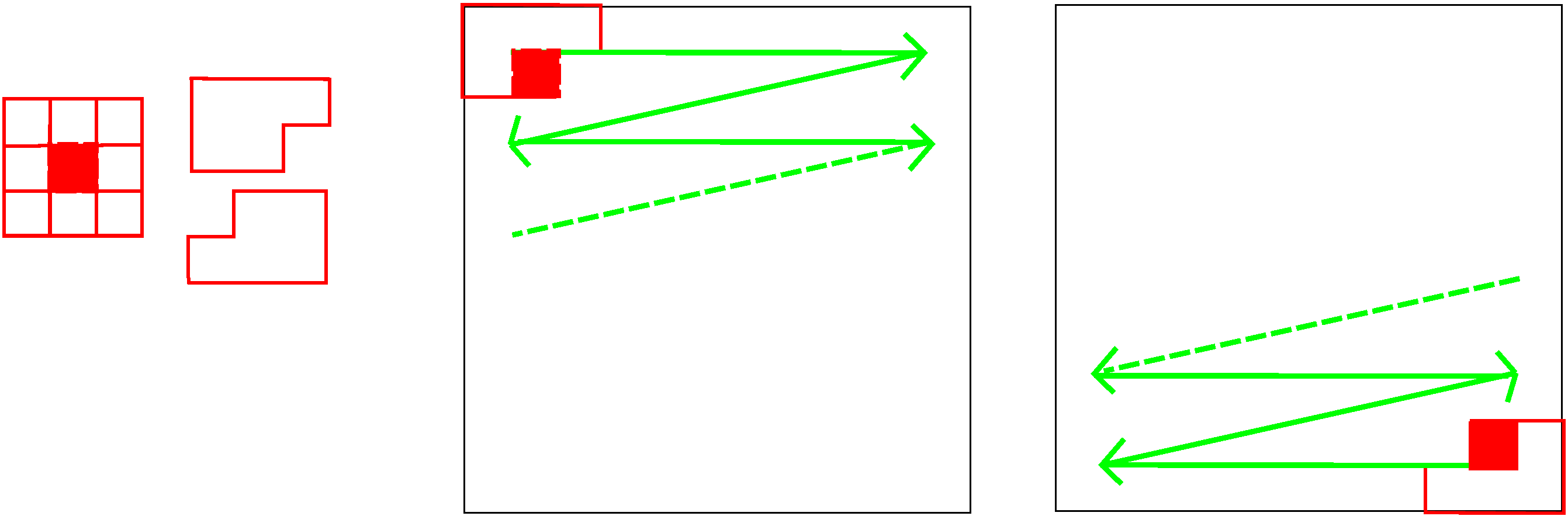
Elementary Chamfer Masks 
Also true for  with the following rewriting rules of the DT map:


Other path-based distances: Look-up table approach


 is the neighborhood test.
Bottlenecks Efficient computation of Lut, bounds on  , bounds on
  , …
, …
Idea
Get the Medial Axis as a by-product of the Power map
Lemma
Let  and
and 
Non-empty power map cells are related to maximal balls
[Skipping details…]
 Separable algorithm to extract the medial axis
computational cost for a large class of metrics
|
|
|
|
|
|
Question
Is the set of maximal balls a minimal representation of X as union of balls ?
Answer No
Toward minimal MA
Thm.
If we allow k-ary predicates  with
with
 the minimal medial axis problem becomes
NP-complete
the minimal medial axis problem becomes
NP-complete
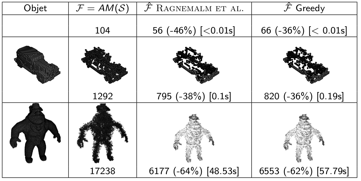
Digital Medial Axis is defined as a set of balls without any topological information
We are thus looking for
Iterative thinning via Simple Point Removal
Def.
A point is simple for if and  are in the same homotopy equivalence class
From Simple Point Definition
Let  by any sequence of insertions/removals of simple points, then and
  are in the same homotopy equivalence class
How to characterize simple points ?
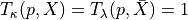
 -simple points§
Definition
Def.
A point is  -simple for if
and have the same number of  -components
 and
and  have the same number of
  -components
Example
(which are resp. (0,1)- and (1,0)-simple ?)
Main Results
Thm.
In dimension 2 and 3, -simplicity of  can be decided locally at
( neighborhood in 2D,
  )
)
E.g. 2D
 : 8-neighborhood around (without p)
 : set of -connected components in adjacent to

is
-simple for

In dimension 3,  definition is a bit more complex but still local
All configurations in 2D
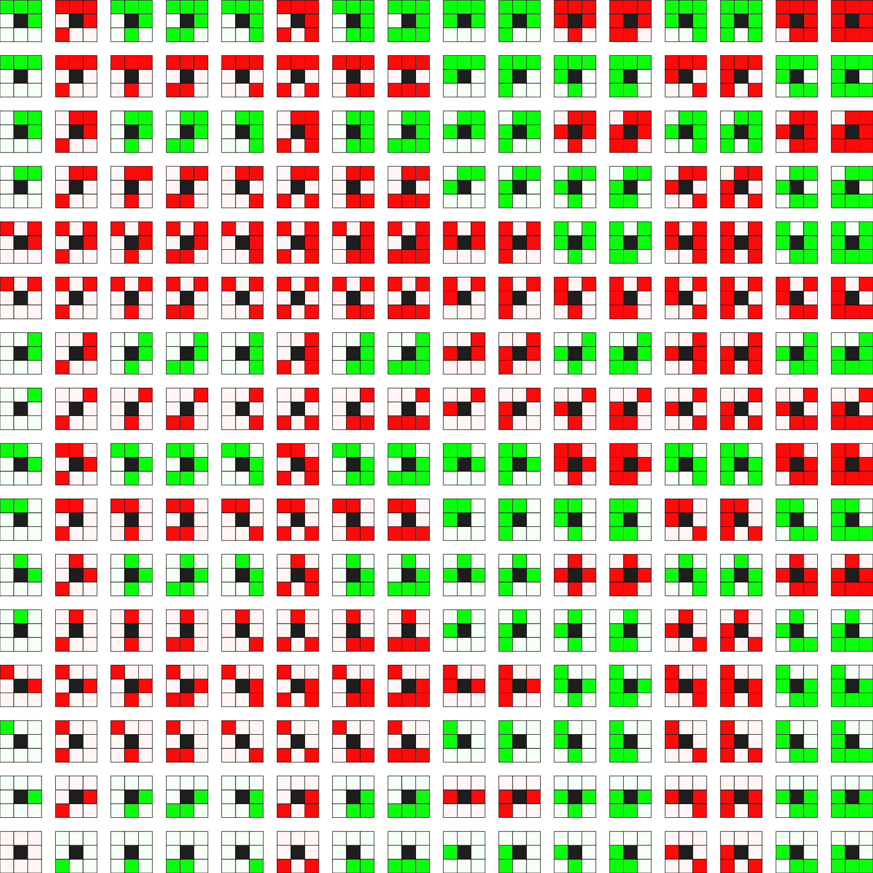
|
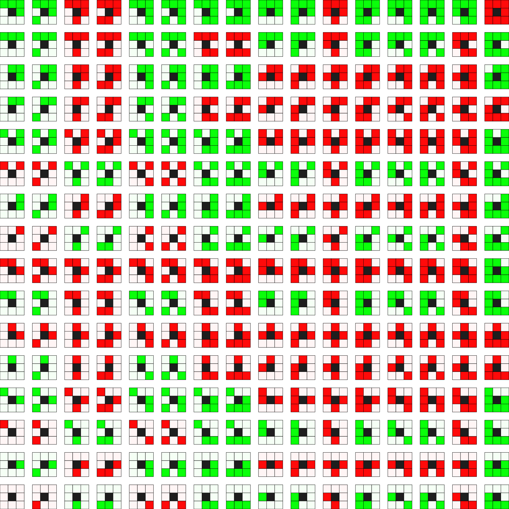
|
| (0,1) | (1,0) |
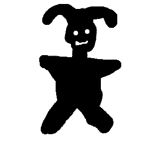
Idea
Iterate until stability over sequential simple points removal ultimate homotopic thinning
|
|
|
|
P = { p in X | p is simple for X }
while ( P != empty )
   Q = emptyset
   for all points p in P
     if (p is simple for X)
       X = X \ {p}
       for all q in N(p)
          Q = Q + {q}

   P = emptyset
   for all points p in Q
     if (p is simple for X)
       P = P+ {p}
Idea
Based on an Oracle, we decide to block some simple points during the thinning
Generic algorithm
Breadth first thinning if P is implemented as a queue
P = { p in X | p is simple for X }
while ( P != empty )
   Q = emptyset
   for all points p in P
     if (p is simple for X) and (p is not anchor point)
       X = X \ {p}
       for all q in N(p)
          Q = Q + {q}

   P = emptyset
   for all points p in Q
     if (p is simple for X)
       P = P+ {p}
E.g.
p is anchor point if it has only one neighbor in X
|

|
Idea
Anchor points can be specified to generate surface based skeleton
|
|
Guided Thinning
Instead of using a queue for P, we consider a priority list with distance transformation values
Better geometry (central axis) of the skeleton
Parallel thinning
usually, parallel thinning algorithms are more efficient and provide centered skeletons
Active works
![f(x,y)&=0\\
\vec{g}(x,y)&=(I_x,I_y)^T\\
\vec{t}(x,y)&=\frac{(-I_x,I_y)^T}{\sqrt{I_x^2+I_y^2}}\\
k&=\frac{-t^THt}{\|\vec{g}\|}, \quad H=
\left [ \begin{array}{cc}
I_{xx} & I_{xy}\\
I_{yx} & I_{yy}
\end{array}\right ]](_images/math/0f79b05e3a5beb38567d8b1115315e84c5e36892.png)


![X = \left \{ (i,j)\,|\, \exists k\in[1,N] \, (i - x_k)^2 + (j-y_k)^2 \leq r_k^2\right \}](_images/math/7b82f02081fd75e71a03991842c9f4da1f6406b4.png)