Introduction to Image Processing§
| author: | David Coeurjolly |
|---|
| author: | David Coeurjolly |
|---|
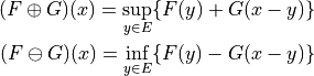
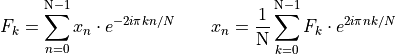
We only focus on values of the functions 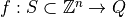 using stochastic
representation
using stochastic
representation
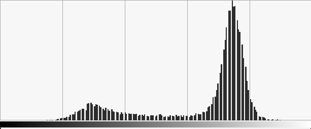
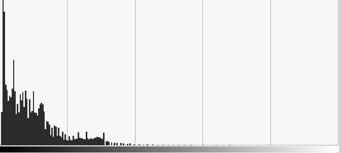
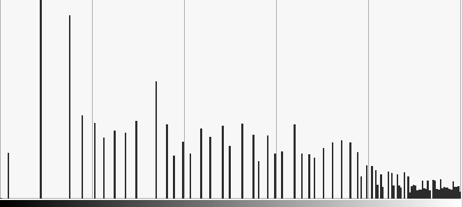
Important object: histograms
The image can be seen as a random variable with probability density
function 
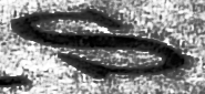
Exemple: ![S=[0,185]\times[0,85],\, Q=[0,255]](_images/math/b4a6c7cfb568ef56cacb9ce5e09003ce34930b06.png)
|
|
Histograms sum up colorimetric information of the image without considering spatial relationships.
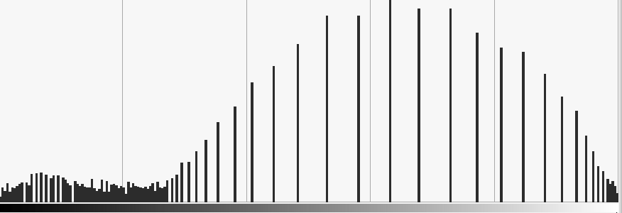
Few examples:
Translation
Histogram remapping
![\,l: [a,b]\subset[0,1] \rightarrow [0,1]](_images/math/7b7df21e0a3ebe7ac0e5b9ee87ee0b2376ee1264.png)
Inversion
…
More generally
Propagation to image  <demo>
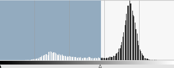
In previous examples,  was prescribed. Now, we are looking
for to map histogram
(empiric or observed) to
was prescribed. Now, we are looking
for to map histogram
(empiric or observed) to  (model).
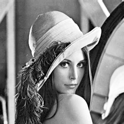
Example: Equalization
: uniform distribution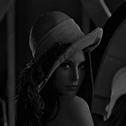
|
|
|
|
Be careful not always a good idea
|
|
Image Segmentation classify pixels into classes such that intra-class pixels share the same visual properties (colorimetric information, geometrical properties …)
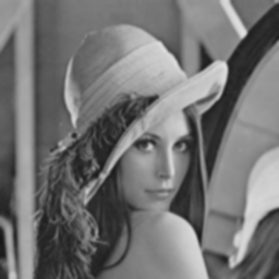
Let’s go back to initial image:
|
|
|

|
|
Histogram Thresholding
<slides>
Take into account spatial relationships between pixel values
Key tool: convolution
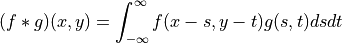
Image as a function 
We consider the result of the convolution product of  by
by 
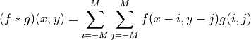
or a discrete version for compact support kernel 
Algorithmically
Direct discrete computation of the support is small
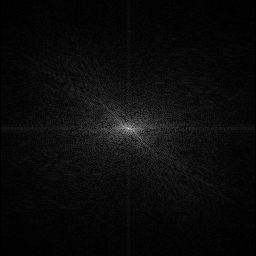
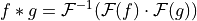
Or by regular product on Fourier space:

|
|

(for  )
)
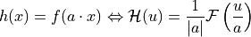
Linearity 
Scaling
Transaltion

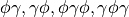
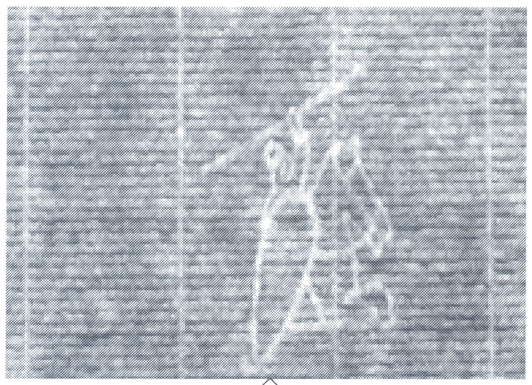
Modulation for real 

Convolution

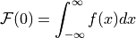
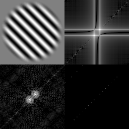
DCT component
(magnitude of Fourier transform leads to translation and rotational invariant descriptors)
(http://www.cs.unm.edu/~brayer/vision/fourier.html)
|
|
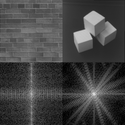
|
| Pure cosine signals | Magnitude vs. Phase | Real image example |
(http://www.cs.unm.edu/~brayer/vision/fourier.html)
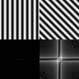
|
|
| Continuous vs. discrete FT | Edge effect reduction through convolution |
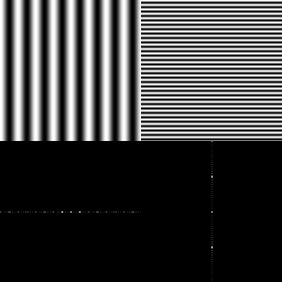
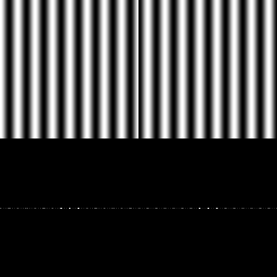
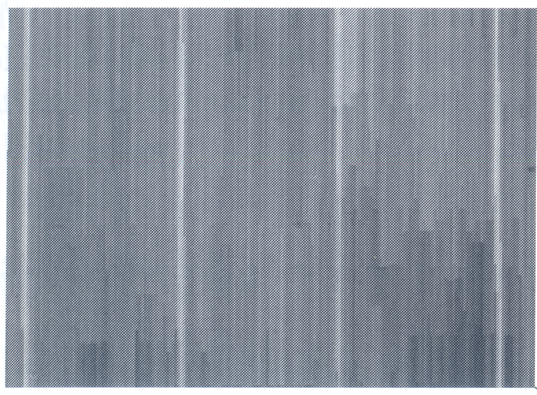
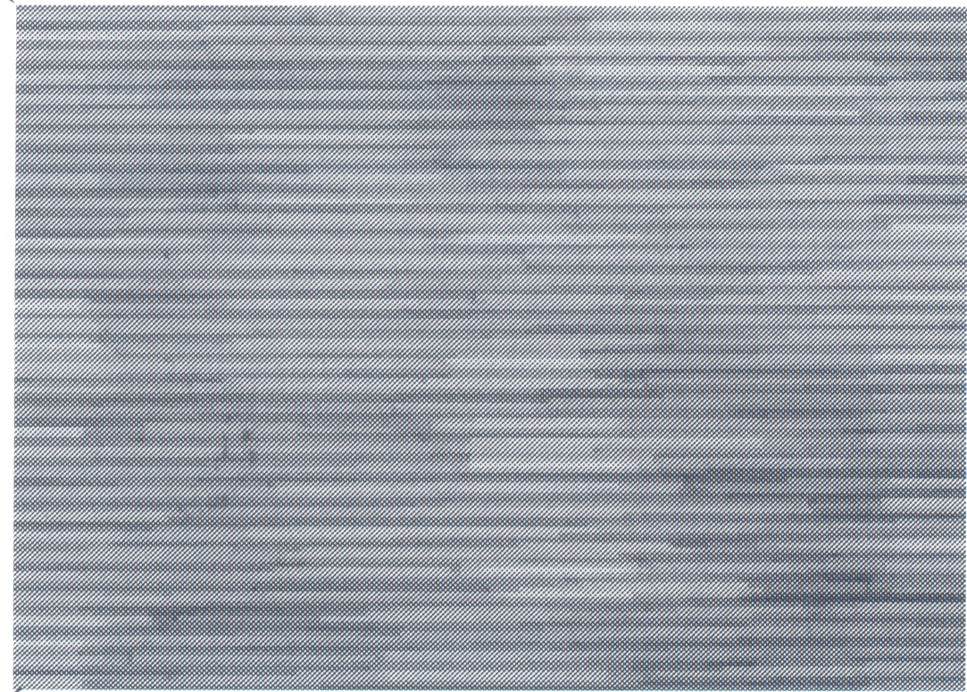
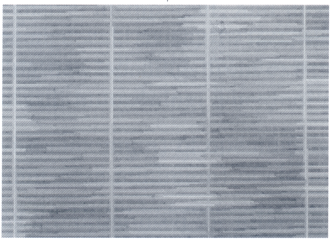
Periodic structure:
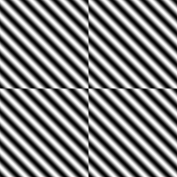
(http://www.cs.unm.edu/~brayer/vision/fourier.html)
|
|
| Lowpass filter | Highpass filter |
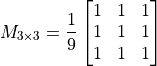
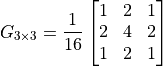
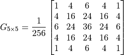
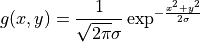
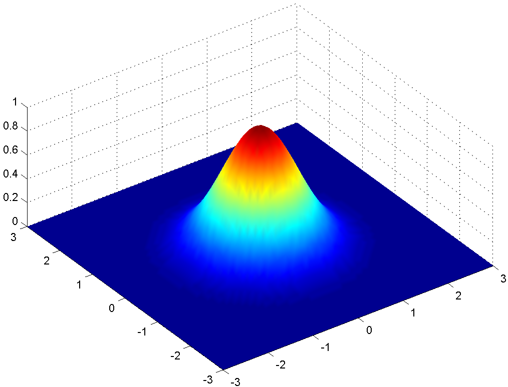
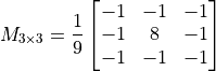
Smoothing / Low-pass filters
G : Gaussian kernel approximation function
 binomial coefficients, ….
 |
|

|

|
 |
|

|

|
 |
|
|

|
Match between filtering and noise model
| Gaussian noise | 
|

|
| Specular noise salt/pepper | 
|

|
| Contour spread | 
|

|
Complementary filters to low-pass filters
|
|
|
Median filter

15
…but…
complexity for a size  domain?
|
|

|
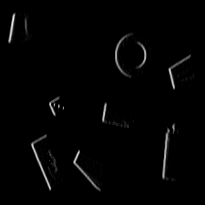
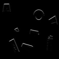
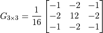
Context
loci if high gradient vector norm of the function 
Zero-crossing of the Laplacian  …
…
|
|
We will focus later to segmentation process.
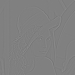
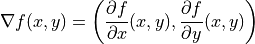
Definition
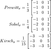
Finite difference approximation
(other masks exist along specific directions  )
)
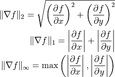
Amplitude = gradient vector norm
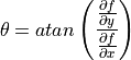
Orientation
a contour can be characterized has pixels with
high gradient vector norm
|
|
|
|
(Prewitt)
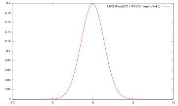
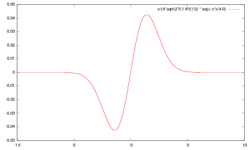
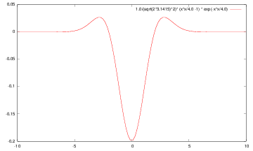
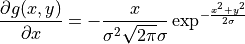
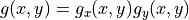
Gradient of ta filterer image and Gaussian smoothing filters
let us consider Gaussian kernel filter 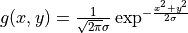 ,
we have
,
we have
|
|
|
| g | g’ | g’‘ |
Let  be a convolution filter (
 Impulse
response of a filter). The filter is separable if
Impulse
response of a filter). The filter is separable if
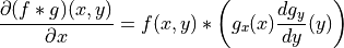
Thus:
and for partial derivatives:
direct consequences when implementing filters
(only 1D convolutions)
![g=[1\, 1 \,1]](_images/math/d5c151ac1aed07cf60f932711e26ab05cb24632a.png) and
and ![d = \nabla h = [-1\, 0 \,1]](_images/math/37175632cc856a1de6949ab919270fe53ecf6104.png) then
then 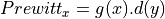
i.e. Prewitt’s filter corresponds to finite difference approximation
of the result of a constant smoothing filtering of
Canny’s criteria (1983)
Noise model + signal model + Criteria modeling + initial conditions
Optimal filter as solution of a PDE
|
|
Shen-Castan :  |
Deriche :  |
The Gaussian filter is a good approximation of such optimal filters
Contour extraction requires gradient vector norm (or zero-crossing laplacian) thresholding
Naive approach:  belongs to a contour iff
From hysteresis : belongs to a contour iff
or
 and
and  neighbor of
  such that
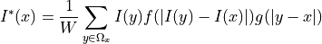
[Tomasi & Manduchi, 98]
Non-linear filter with a pair of spatial intensity kernels

 is a window around
  and are decreasing functions
![[0,+\infty]\rightarrow\mathbb{R}^+](_images/math/f43e23d89fb1a0676a1adb79beb6190213cd50a8.png) (e.g. Gaussian kernels)
(e.g. Gaussian kernels)(From [Bilateral Filtering: Theory and Applications Sylvain Paris, Pierre Kornprobst, Jack Tumblin, and Frédo Durand Foundations and Trends in Computer Graphics and Vision, 2009])
Question: How to efficiently implement bilateral filtering ?
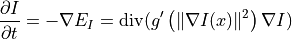
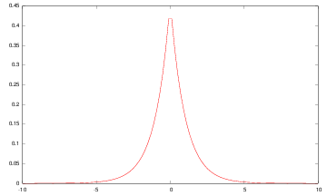
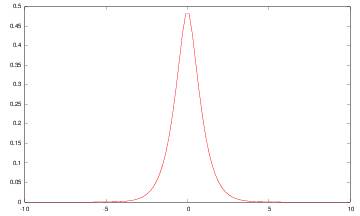
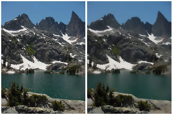
[Perona, Malik]
Images as functions 
Diffusion process defined on time-varying images: 
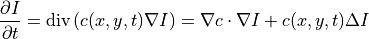
with for example:
Anisotropic diffusion process that removes noise preserving edges
Rationale: for some  we want
to minimize
we want
to minimize
and thus
|
|

|

|
N.B Bilateral filtering is asymptotically close to Perona-Malik’s diffusion
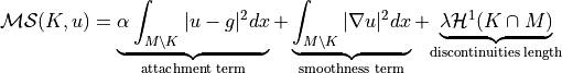
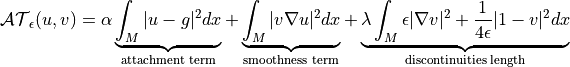
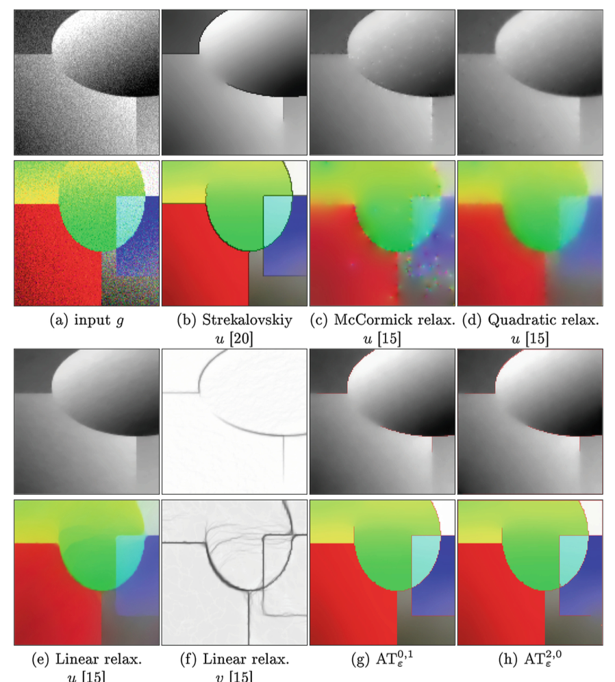
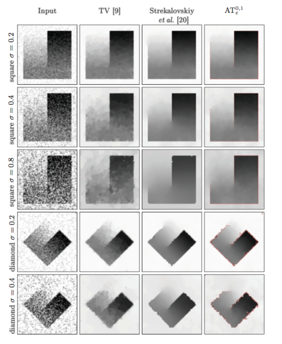
Idea Variational formulation edge aware smoothing
 is the function domain
 is the input raw image
 is the regularized image
 is the discontinuities support set
 is the Hausdorff measure
But:


 has to be optimized
 convergence mathemtatical framework
:-)
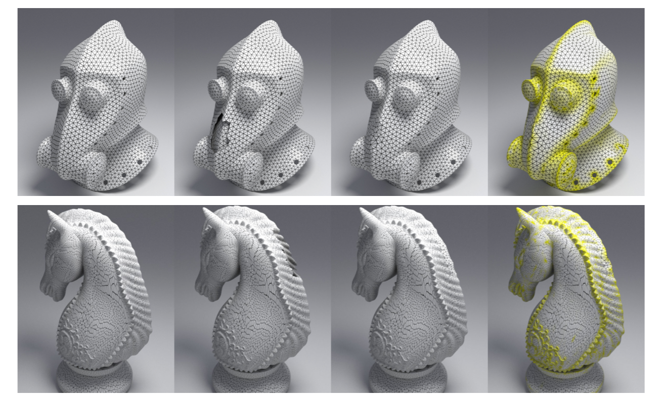
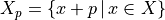
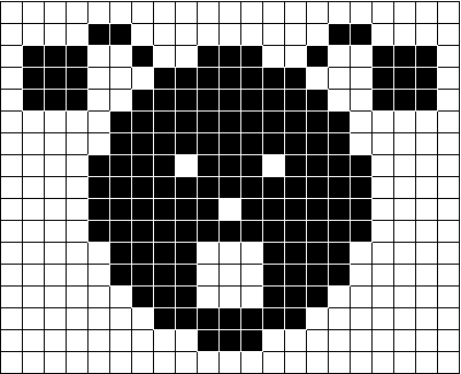
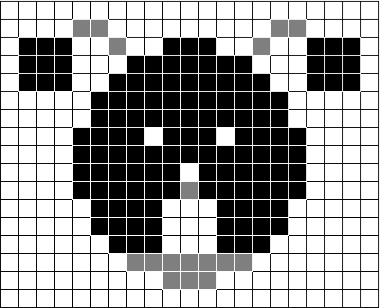
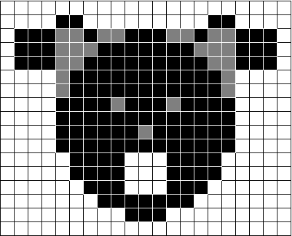
[Matheron, Serra, …]
Idea

Translation
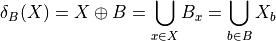
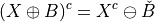
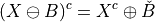
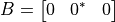
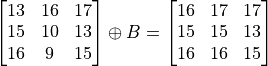
Dilation by a structuring element B
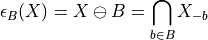
Erosion by a structuring element B
Properties
with  and
and 
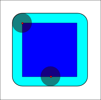
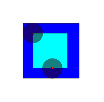
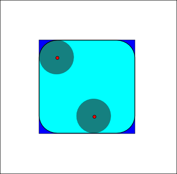
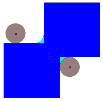
Structuring element: Euclidean disc
|
|
(blue: set  , gray circle: structuring element and cyan: result of the operators)
Opening B
Closing
|
|
3x3 structuring element
|
|
|
Properties
Opening is anti-extensive: 
Closing is extensive: 
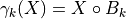
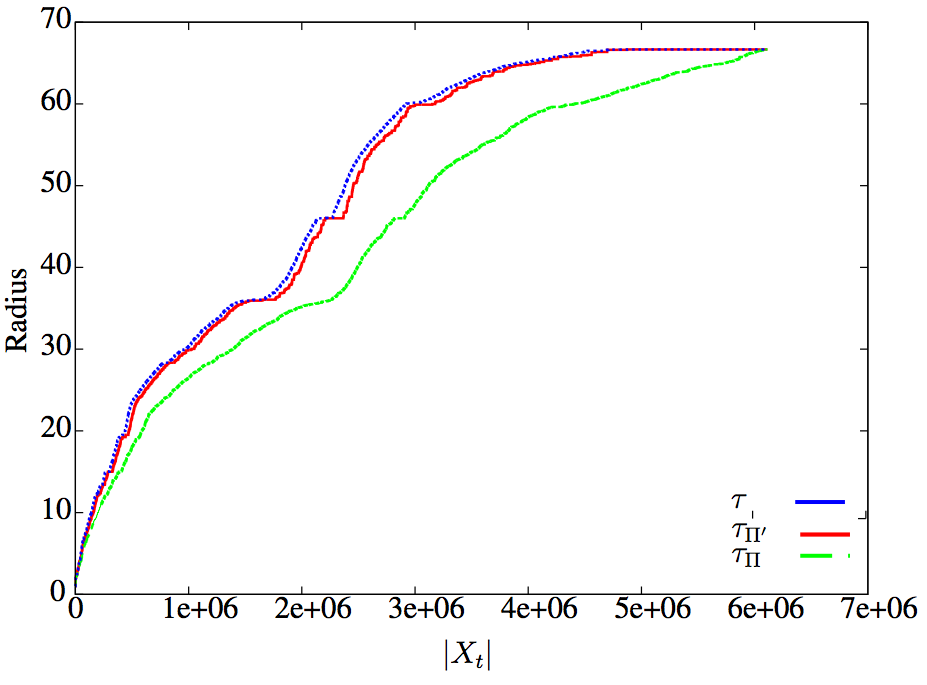
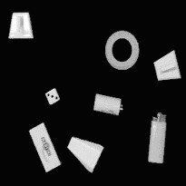
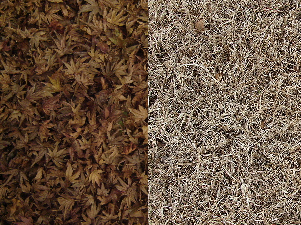
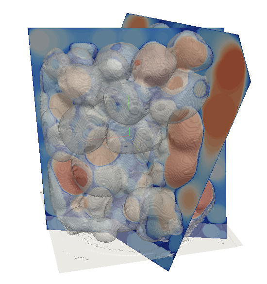
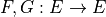
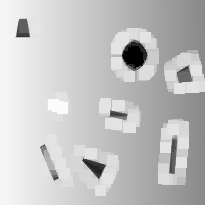
Useful tool for granulometric analysis
Sequence of increasing structuring elements  k times
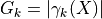
 is called the granulometry function of and
  the spectrum
Intuitive explanation
is defined as the union of grains and is the size of the set  defined by grains larger than k
|
|
|
|
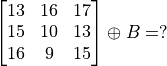
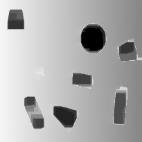
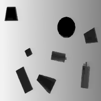
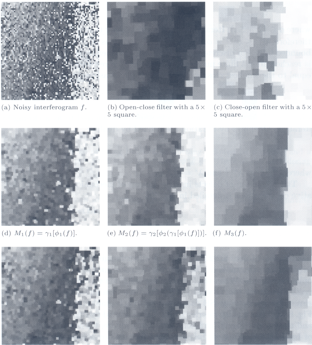
Operators on gray-level images
Example
Let suppose a grayscale image and a constant structuring element (whose origin is it mid-point, so-called flat structuring element)
Then

|
|
|
|
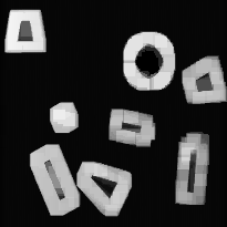
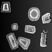
Basic “à-la” finite difference definition
Gradient
Laplacian
|
|
Mathemtatical model
Operators acting oncomplete lattices

Principle
Given an specific image
Select the best structuring element(s)
Specify the combination of fundamental operators (e.g. series of opening/closing)
 is a filter iff it is increasing and idempotent
 are filters
 are
filters and
are
filters and
|
|
|
|
[Soille]
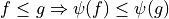
![H: Q \rightarrow [0,1]](_images/math/82b33313868c14f9d85eab0b4fd163f9de1777f1.png)
![\phi: [0,1] \rightarrow [0,1]](_images/math/6c24c45b00c43d662c2e8d6bbf857d78dd1fa307.png)


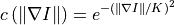
![E[I]={\frac {1}{2}}\int _{{\Omega }}g\left(\|\nabla I(x)\|^{2}\right)\,dx](_images/math/5361f56602dd380c553a193f12cd3b6dba9347d8.png)