Image processing basics

This notebook introduces basic notions and tools for image processing : color representations, image models, histogram manipulation, linear filtering via convolution and fourrier domain analysis, some non linear denoising.

Table of contents

Python libraries and code to illustrate this course, you can safely read this later if you are interested

Images

Perception

Images aim at storing what our eyes see. We therefore need a better comprehension of what we see to understand how we can store it. Vision is the process through which our eyes collect the electromagnetic radiation circulating in our environment and interpret it to get a representation of our surroundings. What we call visible light is the set of electromagnetic radiations that our eyes can perceive.

To perceive light, our eyes are equipped with several types of photosentive cells, mainly rod cells and cone cells. Rod cells are mostly responsible for low light vision, while cone cells allow us to perceive colors. Cone cells can be divided in three groups depending on the set of wavelengths they react to. S cells are activated by small wavelengths (around blue), M cells for medium wavelengths (around green) and L cells for long wavelengths (around red). The following image (courtesy of Wikipedia) details the reaction of these cells as a function of the wavelength.

cone cell reaction (courtesy of Wikipedia)

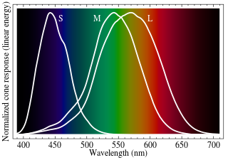
The distribution of these cells vary between individuals, but we are mostly equipped with M and L cells. Some classical diseases impact this distribution, such as color blindness usually due to some type of cone cells missing.

The perceived color of an object corresponds to the light we receive from the object. Unless the object is itself a light source, this light usually commes from the reflection of the light emitted from other sources. The material of the object absorbs some parts of the spectrum and reflects some others. Determining the color of an object therefore amounts to determining this absorbtion function. We however usually perceive the object under specific light conditions. Our brain is therefore responsible for estimating the lighting conditions, and deducing the color of the object. This process however varies between individuals, and when dealing with pictures taken with a camera and displayed on some other medium, people may interpret color in different ways. A classical example is the following picture (source unknown, taken from the Times of India), which received a bit of fame on social media

grey pink shoes (courtesy Times of India)

Depending on your brain reaction, you can perceive this shoe as grey with green laces, or pink with white laces. If you look at it for a longer time, you might end up enterpreting it in the right way, which is pink and white. The reason for this is that the picture was taken with a green ambient light. Looking at this picture out of context makes it more difficult to guess the ambient lighting conditions, and therefore the actual color of the shoe. In terms of the stored data, without interpretation, the color is grey.

Color reproduction and representation

Storing images is pointless without means to reproduce them. To reproduce an image, a device has to recreate an excitation of the eye cells in order to mimic the excitation perceived at the moment the image was taken. Two main families of methods exist for this purpose. Additive synthesis uses light emitters specifically designed to trigger the groups of cone cells individually. This type of synthesis is typically used in screens. Subtractive synthesis filters an input white light source with filters specifically designed to reduce the excitation of each family of cone cells. This is especially used in printing devices.

RGB colors

When dealing with additive synthesis, as seen on the excitation curves of the cone cells, we know the wavelengths triggering each family of cone cells. Roughly, the S family is excited by blue light, the M family by green light and the L family by red light. The display device therefore exhibits a distribution of tiny light emitters : red, green and blue ones. To pilot such a device, one has to provide the intensity with which each of these emitters should function. The naïve RGB model therefore stores these three intensities as numbers, ending up with a three dimensional color space.

CMYK colors

A printed document is a subtractive synthesis device. Assuming the document is printed on white paper and lit with white light, the document is covered with layers of semi-transparent inks. The incoming light goes through the layers of ink and bounces on the white paper. The paper being white, it does not alter the spectrum of the light. The light then traverses the inks layers once again to finally reach our eyes. Three inks are used, one to tone down the wavelengths of each cone family. Cyan, magenta and yellow are used to filter out their respective complementary colors : red, green and blue. To save color inks in printers, a fourth black ink is generally used to tone down all wavelengths simultaneously : black. Printing using this set of inks is called quadrichromy. The color is represented with four numbers corresponding to the amount of each ink required.

On the figure above, the three ink colors cyan, magenta and yellow can be seen on the corners of the cube opposite to the color they filter. Cyan is diagonally opposed t red for instance.

Other color spaces

The two color spaces presented above are directly related to display devices. These devices are however not able to synthesize every visible color. The portion of the set of visible colors that a color model is able to represent is called its gamut. Many other color models exist with various applications. Some are based on capture devices rather than display devices and camera manufacturers have proprietary formats to store the light measured by their sensors. Pictures taken in RAW format store the sensor data without alteration. Other color models are meant to enhance user experience when manipulating colors. For instance the HSV color model allows an artist to define a color first by its hue, and then from this hue adjust the "saturation" and the "value" of the color. The LAB model aims at defining a color space where measuring the euclidean distance between two colors gives a correct estimation of the perceptual difference between the colors for an average human.

The take home message here is that all color models are not equivalent, and depending on the use case some might be better than others. Conversion is usually not a bijection. For instance designing a document in RGB requires a conversion to CMYK before printing, which may alter the resulting colors.

Storing images

Depending on the context, there exists many ways to store images. These data structures are usually split in two families. Raster images store images as a 2D dense array of color values. Vector images describe a process to construct the image using sets of primitive shapes.

Vector images

Vector images can be viewed as one of the earliest formats due to the emergence of display technologies. The first displays were based on cathodic tubes : a beam of electrons was shot and oriented through electric charges to hit a surface at a desired position. The surface was coated with a substance emitting light when hit by electrons. This technology was used in oscilloscopes or radar systems for instance. Vector displays were designed based on this technology, and producing an image on such a display amounts do providing a path for the electron beam. An example of such a display system is the Vectrex console released in 1982 (image courtesy of Wikipedia). Note that at the time, raster displays already existed.

vector screen : Vectres console

Basically vector images can be viewed as a sequence of instructions for a program to draw the image. The image is described in terms of primitives : segments, paths, curves, polygons, glyphs (letters) and so on. A modern example of a standard file format is the SVG (scalable vector graphics) format for instance, but actually a text file also decribes an image in terms of a sequence of glyphs. The PostScript format and its successor, the PDF (Portable Document Format) were designed to describe printable documents in portable ways, and many printers are driven using these formats. The HTML+CSS formats describe web page layouts for your web browser to render, which is also in a way some form of vector graphics.

The main interest of vector graphics is that there is no notion of resolution. The steps to draw the image can be reproduced at any size without some sort of staircase appearing (aliasing).

Raster images

When capturing a picture of the real world through a camera, guessing that some shape is actually a Bézier curve with some set of parameters is a difficult problem. Early cameras didn't even store their images in terms of bits for a computer to process. Early photographs were taken by exposing to light plates with a photosensitive coating. The support of the photograph was therefore a 2D distribution of photosensitive elements. Modern cameras replace this process using a 2D array of sensors. Storing such images is therefore naturally done using a 2D array of color values. Each value is called a pixel (Picture element). Raster images are therefore made of a 2D array of pixels. Each pixel is given a color in the desired color model. This color can be encoded using various levels of precision. For memory reasons, early images encoded color on 8 bit values, therefore only 256 colors were available. The number of bits per channel was correlated with our perception sensitivity : 3 bits for red, 3 for green and 2 for blue (we have fewer cones for wavelengths around blue). Nowadays, most images will use 32 bits per pixels, 8 bits for each red, green, blue chanel, and 8 more bits for transparency (alpha channel). This raw representation is then compressed using various methods.

The image below is an example of a raster image. It's a picture of the city of Reine in Norway.

Raster images are defined up to some resolution. When the resolution is insufficient with respect to the display medium, the pixels become individually visible. In addition, the resolution has to be sufficient with respect to the frequency of the captured phenomenon. This is the well known Shannon Theorem. Basically, when sampling uniformly a high frequency signal with an insufficient resolution, the result may exhibit wrong frequencies.

We see above that the orange dots corresponding to a low frequency sampling of the high frequency signal give the impression of another frequency. Visualy, such wrong frequency are referred to Moiré effects when happening on images. The following image (courtesy of Wikipedia) exhibits an example on the garage door.

Moiré effect

In the following course, we focus on processing raster images. Most of the treatments below are useless in the case of vector images : separating objects from background is trivial for vector images since the background will usually be a separate primitive, preserving edges is not a problem since different objects are described by different primitives. Converting a vector image to a raster image is called rasterization. Its complexity depends on the primitives used, but it's usually simple and fast.

Global filtering

Global filtering processes images based on global metrics on pixel values, colors and distribution. The operation is performed globally on the image, without trying to detect and preserve local structures.

Grayscale conversion

Grayscale conversion is a perceptive problem : conversion from colors to luminance. A naive approach would be to use the mean of the RGB values as luminance.

This approach however does not conform to the human perceptive system, and some areas are not properly rendered. For instance on the island on the left, too much contrast is present between the shades of green, whereas in the sea, the different shades are greatly diminished. Based on perceptive studies, coefficients have been derived to convert the RGB values into luminance. Basically, the perceived luminance is mostly due to the red and green channels and blue has little effect on the result.

You can find below the comparison between the two approaches, and try to determine if the perceptually based conversion suits you best.

Thresholding

Thresholding is a classical technique to try and extract elements from images. We show below how to try and seperate the background from the objects on the picture. The idea is to define a value (the threshold) and filter the pixels depending on whether their value is above or below the threshold.

finding the correct threshold is not trivial, since it will depend on the lighting conditions when the picture was taken, and on the background and objects themselves. A method to try and determine automatically a threshold is to study the histogram of the image. The histogram aggregates for each possible value the number of pixels containing that value.

We see here several groups of shades as bumbs on the histogram. We can now try and seperate these groups by choosing a threshold in a valley between peaks. For instance 155 here.

Even though some noise remains, we can hope to process further this result to extract the objects, using for instance connected components, filling holes in them and removing smaller ones.

Normalization

Studying histograms can provide insight on how to improve and process images. Normalization aims at detecting portions of the spectrum that are not used, and rescales the shades to span the entire area. Taking the landscape picure above in grayscale, we get the following histogram :

we can see here that shades below 50 are not used. We can scale the shades to widen the histogram and make a better use of the dynamic range at our disposal.

Equalization

Histogram equalization pushes further the usage of the dynamic range of the shades. It moves the shades so that each available shade has approximately an equal contribution to the image. The target histogram would therefore be a flat line. To do so we start by studying the cumulative sum of the histogram. This shows the amount of pixels in the image having a shade below some threshold.

Now the desired histogram would be flat, and the corresponding desired cumumative sum would be a line :

Given an input shade, using the original cumulative sum, we can determine the number of pixels below this shade. Now mapping this number of pixels on the y axis of the desired cumulative sum, and using the line to determine the corresponding shade, we obtain the corresponding shade in the target image.

Linear filtering

Many image processing techniques are based on linear filters and convolution. The idea is to compute the target image as the convolution between the input image and a kernel. Using a linear filter can be done efficiently using the Fourrier transform : both the image and the filter can be transformed in the frequency domain. In this domain the the convolution becomes a multiplication which can be easily performed, and the resulted is converted back into the spacial domain.

Convolution

Mathematically the convolution of the function $f$ with the kernel $g$ is defined as :

$$ (f*g)(x,y) = \int_{-\infty}^{+\infty}\int_{-\infty}^{+\infty} f(x-s, y-t)g(s,t)\mathrm{d}s\mathrm{d}t $$

When using images, these integrals reduce to sums. Assuming the kernel is defined on the integer grid $[-m, m]^2$, we get the sum :

$$ (f*g)(i,j) = \sum_{s = -m}^m\sum_{t=-m}^m f(i-s, j-t)g(s,t) $$

The kernel can be seen here as the influence of a pixel in its neighboring pixels in the resulting image. For each pixel, the kernel is multiplied by its value and splat, centered at the pixel, in the resulting image. The result is the sum of those splats. Changing the order of the summation, the result can be computed as a sum of shifted versions of the images. For each coefficient in the kernel, the original image is multplied by the coefficient and splat in the result, shifting it with an offset opposite to that of the coefficient wrt. the center of the kernel. Using an opposite offset flips the kernel, so that it corresponds to the influence of the neighboring pixels at a central pixel, rather than the influence of a central pixel in its neighboring pixels.

On the edges of the image, the nearest pixel value is usually taken when no pixel is available.

Blur

Average filter

This filter replaces the value at a pixel by the average of color of the neighboring pixels. This filter smoothes the sharp features in the image. Each neighboring pixel in the surrounding window has the same influence. Using a 9x9 window for instance, each pixel has the influence 1/81.

Zooming the image, we can see that the shape of the window can create visual artifacts in the result. Here, the fact that the window is square creates visible horizontal and vertical halos around the sharp features of the image.

Using a circular window reduces these artifacts.

Gaussian filter

The gaussian filter reduces artifacts that can appear using the averegare filter, because of its sharp transition between pixels used and not used in the average. Using the gaussian, the further the pixel is from the center of the pixel, the smaller its influence.

A 2D gaussian is defined as

$$ G: \mathbf{x} \mapsto \frac{1}{2\pi\sigma^2}e^{-\frac{\lVert \mathbf{x} - \mathbf{\mu} \rVert^2}{2\sigma^2}} $$

Where $\mathbf{x} \in \mathbb{R}^2$ is the evaluation point, $\mathbf{\mu} \in \mathbb{R}^2$ is the center of the gaussian (the mean of $\mathbf{x}G(\mathbf{x})$) and $\sigma$ its standard deviation (controlling how flat the gaussian is). The $\tfrac{1}{2\pi\sigma^2}$ factor ensures that the integral of this gaussian over $\mathbb{R}^2$ is 1.

Gaussians have an infinite support, meaning that they are strictly positive everywhere. It terms of linear kernels this would mean that any pixel influences any other. In terms of efficiency, this is can be problematic. However gaussian decrease quickly towards zero and approximations exist with a limited support, the most common using binomial coefficients.

Fourrier domain

Using the Fourrier transform, the image can be represented in terms of frequencies.

The Fourrier transform for a 2D function $f : \mathbb{R}^2 \rightarrow \mathbb{R}$ is a 2D function with complex values given by

$$ F(f)(\nu,\xi) = \int_{-\infty}^{+\infty} \int_{-\infty}^{+\infty} f(x,y)e^{-i 2 \pi (\nu x + \xi y)} \mathrm{d}x \mathrm{d}y $$

with $\nu$ and $\xi$ to be interpreted as frequencies. This decomposes f on the Fourrier basis, which are the functions $e^{i2\pi(\nu x + \xi y)}$, which are oscilating functions with in the direction $(\nu \xi)^t$ and wavelength $\sqrt{\nu^2 + \xi^2}-1$.

When the original function is made of pure wavelengths, the Fourrier transform is just made of peaks at the corresponding frequencies.

Note that to obtain the spectrum above, the fft is shifted to center it in the dft_show function. The shift moves around parts of the spectrum so that the low frequencies are in the center, and the high frequencies towards the sides :

In the case of an image the transform shows the high frequencies in the center and the high frequencies on the boundary.

Low / High pass filtering

A low pass filter removes the high frequencies and keeps the low frequencies. It can be naively done by just setting the high frequencies to zero outside of a centered window.

You can notice that this naive strategy produces riples in the result, emitted from the sharp features in the image.

These ripples happen because sharp features in one domain provoke an oscilatory response in the other domain. Taking for instance a circular window

Looking at the corresponding frequencies, we obtain somehting of the order of a sine cardinal $\tfrac{\sin{x}}{x}$ :

Considering this same window in the frequency domain, and looking at its corresponding function in the time domain also yields oscillations. These oscillation are especially visible at the sharp features of the image, when they bleed on parts of the image with a different content.

Note here that we shifted the result for centering : fast Fourrier transform assumes that the input signal is periodic, and that the origin is at the lower left of the image. When designing kernels for linear image filtering, the origin is set at the center of the image, not at the lower left. Since the result of the inverse Fourrier transform is periodic, we can translate the origin by swapping parts of the domain.

To avoid these ripples, the common good practice is to avoid applying sharp windows on the signal. Gaussian windows are preferred :

The Fourrier transform of a gaussian is actually a gaussian as well :

Multilplying by the gaussian window in the frequency domain therefore discards high frequencies. The gaussian kernel here is inverse shifted since the reine_fft frequency image was not shifted to feature low frequencies at the center of the image.

Since the inverse Fourrier transform of a gaussian is a gaussian, a low pass filter with a gaussian filter is equivalent to a gaussian blur of the image. Note here that on the boundaries of the image, the pixels seem to wrap and you see a thin strip of pixels at the top similar to those at the bottom. When using Fourrier transforms, the input signal (here the input image) is supposed to be a periodic function. This means on our images that neighboring pixels on the top side of the image are taken at the bottom side, and similarly for other edges.

Using the complementary of a gaussian window yields a high pass filter. The high frequencies in an image correspond to its details, where it varies quickly.

Sharpening

A gaussian filter of an image smoothes the details in the image. Therefore substracting the gaussian blur of an image to the image itself yields the details in the image. The sharpen filter uses this idea to recover the details, and then emphasize them.

We see here the details that are extracted using the details filter.

Compared to the sharpened image, the original image now seems blurred.

A convolution in the time domain is equivalent to a multiplication in the frequency domain. Looking at the Fourrier transform of the filter shows that it keeps the low frequencies, but adds more importance to the high frequencies.

We show here that the convolution of the image with the sharpen kernel is equivalent to the multiplication in the frequency domain by the Fourrier transform of the filter.

The translation visible between the input and the output image is due to the 3x3 kernel being impossible to properly center before the Fourrier transform without interpolation and approximation. Rolling the image back one pixel (the half width of the kernel) removes the translation.

Advantages of linear filtering

The main advantage of linear filtering lies in the fact that using the fast Fourrier transform, a convolution in the spacial domain becomes a pixel by pixel multiplication in the frequency domain. The naive implementation of out apply_kernel method above involves a loop on each pixel of the kernel, which sweeps the whole image at each iteration. The resulting complexity is therefore the number of pixels in the kernel multiplied by the number of pixels in the input image. For big kernels this is costly.

The fast Fourrier transform can be performed in $O(n\log{n})$ for an image made of $n$ pixels. Therefore, padding the kernel with zeros to match the resolution of the image, both can be transformed in the frequency domain in $O(n\log{n})$, then corresponding pixels can be multiplied in $n$ multiplications, and finaly the result can be converted back in the spacial domain in $O(n\log{n})$. For big kernels, this is therefore much more efficient.

Note that the time comparison is not entirely fair here, since numpy calls external compiled libraries to compute fft while our naive implementation uses a slow python loop. This however does not compensate for all the additional time spent.

Non linear filtering

Even though these filter do not benefit from the efficient implementation above, in some cases, non linear filters can be very usefull. We show here two examples among many others.

Bilateral filter

The bilateral filter is a gaussian filter which dampens the influence of a pixel on a neighboring pixel whose value is very different. Another gaussian is thus added for this dampening. The implementation below is a naive implementation, more efficient approaches and approximations of this filter exist. The goal of this filter is to smooth regions where colors are similar, but to keep the sharp details in the image.

as desider, we see that regions with similar colors are smoothed, while sharp features are preserved.

Median filter

The median filter is good at suppressing salt and pepper noise. This happens when some pixels have totally wrong values, introducing some kind of grain in the image. Such pixels are sometimes referred to as fireflies.

To cope with such noise, the median filter considers all pixels values in a window around the pixel, and replaces it with the median value.

Noise in rendering

Removing noise can seem to be some synthetic problem when one invents some kind of perturbation of an image and finds a method to remove it. But noise actually happens in real applications. Related to this course, noise can often be found in rendering. In this context, each pixel color is computed as the integral over the pixel area of the light intensity reaching the pixel. This integral is estimated using Monte Carlo techniques : the space of paths reaching the pixel is randomly sampled, and the integral is estimated as a discrete average of the light intensity carried by these paths. In some regions however, paths carrying lots of energy and others only carrying a little reach the same pixel. When insufficient samples are taken, the average yields a noisy approximation of the integral. Taking more samples reduces the problem but requires lots of additional computations. Filtering the noise can therefore cheaply reduce the problem. Here is an example with a cube lit by a square emitter. Using four path samples per pixel yields lots of noise, whereas using 128 samples reduces the noise, but requires much more computation time.

In this case however, althugh it looks like salt and pepper noise, a simple median filter is not sufficient to improve the image. Noise remains and gets more visible. Removing this kind of noise is therefore still one of the main research topics in rendering.

Mathematical morphology

A classical tool for image post treatment is mathematical morphology. This tool is often used to handle binary images after thresholding to improve the result : remove negligible areas, fill small holes and so on. For image processing, its basic operations are therefore initially defined on binary images (black and white) but can be extended on grayscale images or multi channel images. These operations require a structuring element which can be seen as a 2D shape.

Dilation expands the objects in the original binary image using the structuring element. A pixel $p_r$ in the resulting image will be white if there exists a white pixel $p_o$ in the original image such that when centering the structuring element at $p_o$, $p_r$ is white. Considering the binary image and the structuring element as the sets of coordinates of the white pixels, dilation is the Minkowski sum of the two sets. Denoting $I$ the input image and $S$ the structuring element :

$$ I \oplus S = \left\{ i + s, i \in I, s \in S \right\} $$

Erosion reduces the objects using the structuring element. A pixel $p_r$ in the resulting image is white if when centering the structuring element on $p_r$, all the white pixels of the structuring element are white in the original image. Considering the set approach, this is the Minkowski difference of the input image and the structuring element :

$$ I \ominus S = \left\{ i \in \mathbb{R}^2, \forall s \in S, i + s \in I \right\} $$

Based on erosion and dilation, two other operations are defined. Opening aims at removing small or thin elements. It starts as an erosion, to remove small or thin parts. A dilation is then applied to restore the objects at their original shape.

Closing fills small holes in the image by performing a dilation first followed by an erosion.

Using a combination of these tools can be useful in cleaning an original binary image for segmentation problems.

Final remarks

This courses provided a rough overview of basic tools in image processing, and some terminology shared by people working in the field. Modern image processing however makes intensive use of deep learning techniques. The design of the neural networks uses the tools provided above to some extent (convolution layers for instance), and building training datasets may still require somme of the tratments above. However state of the art methods to extract information from images or convert between various representations are often based on deep learning methods. You can for instance have a look at the Pix2pix method which covers a wide range of applications.