Gestion d’un tas

Problématique

Exemple

Tpoint* alloue_point (double x, double y, double z) {
    Tpoint* p = malloc(sizeof(Tpoint));
    p->x = x; p->y = y; p->z = z;
    return p;
}

void libere_point (Tpoint* p) {
    free(p)
}

Rappels: allocation statique

• s’applique aux variables locales
• stockage dans la pile (en anglais stack)
• allocation en entrant dans la fonction/procédure
• libération en sortant de la fonction/procédure
• gérée automatiquement par le compilateur

Rappels: allocation dynamique

• stockage dans le tas (en anglais heap)
• allocation/libération à la demande du programmeur
  • malloc/free
  • new/delete

Besoins

Besoins: gérer l’occupation d’une plage de mémoire (éventuellement extensible)

• réserver (allouer) des zones d’une taille spécifiée (malloc)
• libérer une zone préalablement réservée (free)

Critères:

• rapidité des opérations d’allocation et de libération
• surcoût en mémoire
• gaspillage (mémoire inutilisée sans raison)

Remarques

• Géré par les bibliothèques standards (malloc/free),
• voire par le langage lui même (new/delete),
• parfois de manière implicite (ramasse-miettes).

→ notion étendue de système d’exploitation.

Méthodes

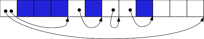
Carte de bits

• le tas est subdivisé en blocs de taille fixe
• on établit une carte: un tableau de bits dont chaque bit représente l’état (libre/alloué) d’un bloc

map:    11000111  11000000  00111000  01111110

limits: 01000000  01000000  00001000  00100010

Avantages

• surcoût en mémoire raisonnable

  exemple : blocs de 8 octets → 1,6 %

  (3,2 % avec les limites)

Inconvénients

• allocation coûteuse en temps (recherche d’espace libre)
• fragmentation interne: certains blocs marqués comme occupés ne sont pas totalement utilisés

→ Peu utilisé en pratique

Liste chaînée

On représente l’état de la mémoire par une liste chaînée dont chaque maillon représente une zone (adresse, taille), son état (alloué ou libre) et pointe vers le maillon représentant la zone suivante.

Évaluation

• La durée des opérations et le surcoût en mémoire dépendent du nombre de zones alouées, et non de la taille du tas.
• Pas de fragmentation interne.
• Permet de gérer des zones allouées contigües.
• L’allocation et la libération sont encore relativement coûteuses (recherche dans la liste, y compris pour la libération).

Allocation

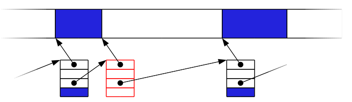
1. On recherche une zone libre de taille suffisante (de taille ≥ à la taille réclamée).

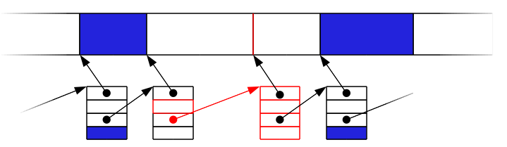
2. On fractionne la zone libre en deux (la première ayant exactement la taille à allouer).

3. On marque la première comme allouée et on retourne son adresse.

Libération

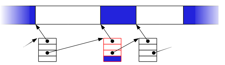
1. On parcours la liste jusqu’à trouver le maillon pointant vers la zone à libérer.

2. On marque ce maillon comme libre. Attention à la fragmentation externe.

3. Le cas échéant, on fusionne la zone libre avec les zones libres voisines.

NB: seuls les voisins immédiats peuvent être libres, donc la fusion ne pénalise pas l’opération de libération (temps constant).

Choix d’une zone libre

Lors d’une allocation mémoire, si plusieurs zones libres de taille suffisante sont disponibles, laquelle choisir?

• Premier trouvé (first fit) : méthode la plus simple et la plus rapide
• Meilleur trouvé (best fit) : cherche la zone libre la plus petite, c.à.d. la plus proche de la taille recherchée.
• Pire trouvé (worse fit) : cherche la zone libre la plus grande.

Avantages ? Inconvénients ?

• Sauf lorsqu’elle trouve une zone de la taille exacte, best fit a tendance a laisser des zones libres trop petites pour être utilisables.
• Worse fit n’a pas cet inconvénient, mais crée plus de fragmentation à terme.
• First fit a l’avantage d’être significativement plus rapide.

Variante 1

Séparer les zones libres et occupées en deux listes.

Variante 1 (suite)

Oblige à maintenir deux structures en parallèle.

Variante 2

Séparer les zones libres par taille.

Variante 2 (suite)

Oblige en plus à gérer les changements de taille.

Méthode Buddy

Principe

Méthode basée sur le principe dichotomique, permettant de diviser la taille du tas par des puissances de 2.

Inconvénients

• fragmentation interne (contrainte sur la taille des zones)
• fragmentation externe

Avantages

• efficace en temps (logarithmique par rapport à la taille de la mémoire)

Fonctionnement

• À chaque taille de zone correspond une liste chaînée.
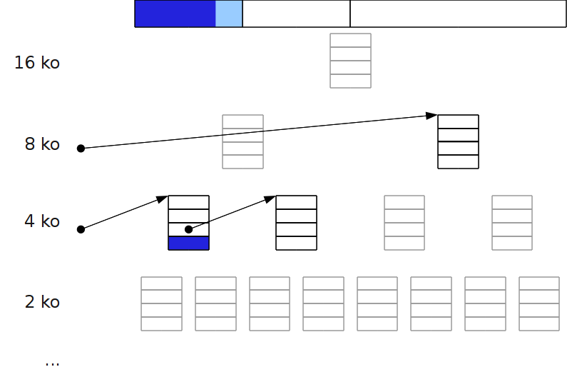
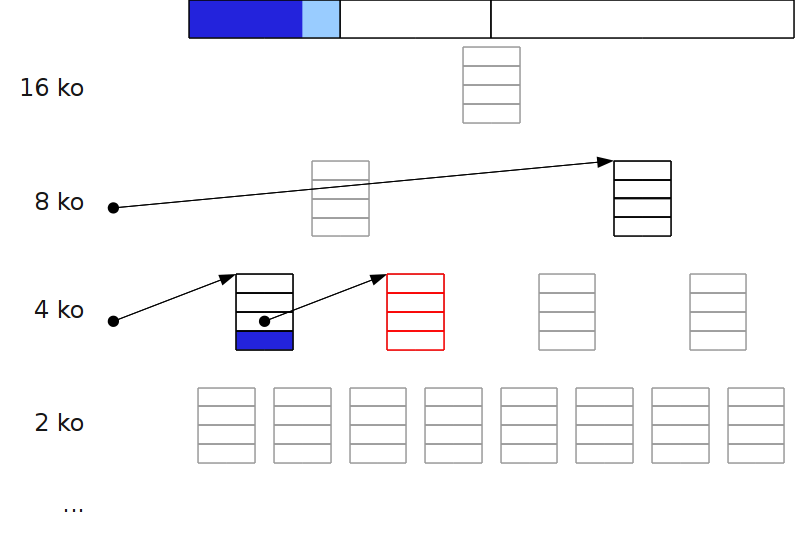
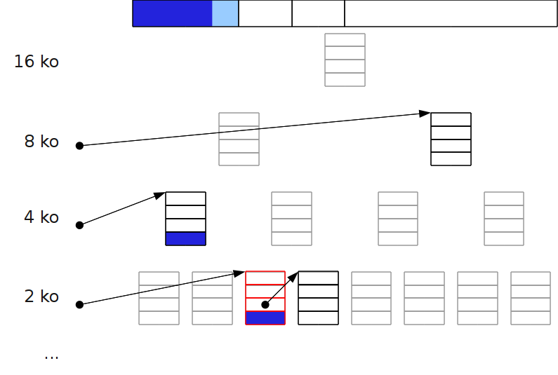
• Allocation : au besoin, on divise par deux une zone libre, jusqu’à atteindre la taille (la plus proche de celle) à allouer.
• Libération : on fusionne deux zones libres si elles sont buddy (« potes ») c.à.d. issue de la division d’un même « père ».

Exemple

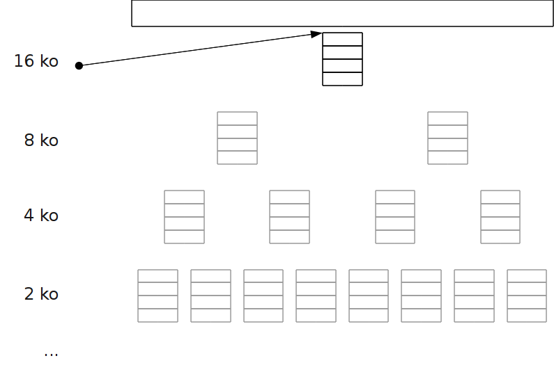
tas de 16ko

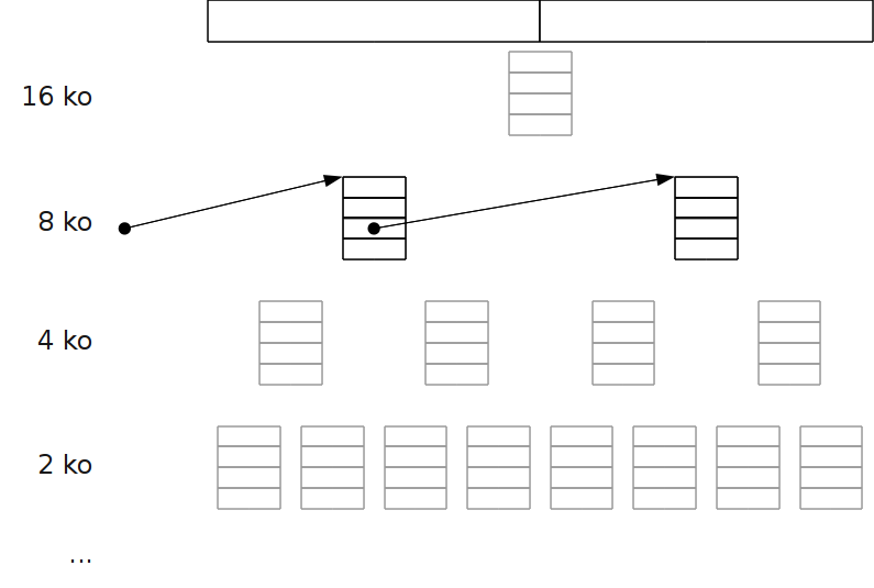
alloue 3ko (1)

alloue 3ko (2)

alloue 2ko (1)

alloue 2Ko (2)

libère zone 2 (1)

libère zone 2 (2)

un peu plus tard

Application

Linux utilise la méthode Buddy pour l’allocation des pages.

→ La fragmentation (interne ou externe) n’est plus un problème puisque

• les pages ont toutes la même taille,
• elles n’ont pas besoin impérativement d’être contigües.

Méthode Slab

• Limitation : toutes les zones à allouer sont de la même taille (structures d’un type particulier)
• Principe : on réserve à l’avance un grand tableau (slab, ou « dalle »).
• On conserve
  • la taille du tableau,
  • une liste chaînée des cases libres.
• Allocation et libération en temps constant.

Illustration

NB:

• aucune référence explicite aux zone allouées.
• le dernier maillon de la liste désigne tout le reste du tableau.

Optimisation

On peut recycler les cases libres du tableaux elles même pour stocker

• l’entête du tableau,
• la liste chaînée,

→ surcoût mémoire minime.

Applications

• Linux utilise la méthode Slab pour l’allocation de ses structures internes (PCB, fichiers ouverts, i-nodes…).
  • Chaque tableau occupe un nombre entier de pages.
  • Pour chaque type de structure, Linux gère en fait une liste de tableaux (buffer) et y ajoute des tableaux au besoin.

Applications (2)

• Utilisable au niveau applicatif

  • pour un type de structure nécessitant de nombreuses allocations / libérations,

  • plus efficace que malloc / free ou new / delete

    → mais attention: pas d’optimisation prématurée.

Extension: ramasse-miettes

Ramasse-miettes

Problème

• La gestion dynamique est une tâche fastidieuse et une source d’erreur (« fuites mémoires ») pour les programmeurs.
• Ceux-ci utilisent par ailleurs des outils informatiques pour les détecter et les corriger.
• Ne pourrait-on pas laisser l’ordinateur gérer la libération de mémoire tout seul?

Mise en œuvre

La plupart des langages modernes (Java, Javascript, PHP, Python, Ruby…) intègrent un mécanisme de ramasse-miettes (garbage collector).

Compteur de références

• Chaque objet possède un compteur de références indiquant combien de liens pointent vers lui.
• Chaque qu’on crée ou que l’on brise un lien vers un objet, son compteur de références est mis à jour.
• Lorsque son compteur de références atteint 0, l’objet est libéré, et ses liens son brisés.

Exemple

Références cycliques

Le comptage des références n’est pas suffisant.

→ nécessité de trouver un compromis entre l’économie de mémoire et le temps de clacul.